サンプルで学ぶ NNabla
このチュートリアルでは、簡単な手書きの数字を分類するタスクを例に、ニューラルネットワークの学習を行うスクリプトの書き方を見ていきます。
注 : このチュートリアルでは、 scikit-learn と matplotlib がインストールされた Python 環境が必要です。
まず、依存関係を準備しましょう。
import nnabla as nn

import nnabla.functions as F
import nnabla.parametric_functions as PF
import nnabla.solvers as S
from nnabla.monitor import tile_images

import numpy as np
import matplotlib.pyplot as plt
import tiny_digits
%matplotlib inline

np.random.seed(0)
imshow_opt = dict(cmap='gray', interpolation='nearest')
2017-06-26 23:09:49,971 [nnabla][INFO]: Initializing CPU extension...
tiny_digits モジュールはこのフォルダにあります。このモジュールは、scikit-learn で利用可能な手書き数字のデータセット ( MNIST ) をロードするためのユーティリティーを提供します。
ロジスティック回帰
まず、ロジスティック回帰のための計算グラフを定義するところから始めます。 ( ロジスティック回帰の詳細は付録 A を参照してください。 )
学習は勾配降下法を用いて行われます。勾配は得られた誤差をバックプロパゲーションしていく ( backprop ) ことで算出されます。
トイ・データセットの準備
ここではこのサンプルで用いるデータセットの準備を行います。
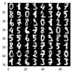
digits = tiny_digits.load_digits(n_class=10)
tiny_digits.plot_stats(digits)
Num images: 1797
Image shape: (8, 8)
Labels: [0 1 2 3 4 5 6 7 8 9]
次のブロックでは、データセットから画像やラベルをミニバッチ分だけ返すデータローダーを作成します。このデータセットはこのサンプル用に利用しているものであり、 NNabla の一部ではないことに注意してください。
data = tiny_digits.data_iterator_tiny_digits(digits, batch_size=64, shuffle=True)
2017-06-26 23:09:50,545 [nnabla][INFO]: DataSource with shuffle(True)
2017-06-26 23:09:50,546 [nnabla][INFO]: Using DataSourceWithMemoryCache
2017-06-26 23:09:50,546 [nnabla][INFO]: DataSource with shuffle(True)
2017-06-26 23:09:50,547 [nnabla][INFO]: On-memory
2017-06-26 23:09:50,547 [nnabla][INFO]: Using DataIterator
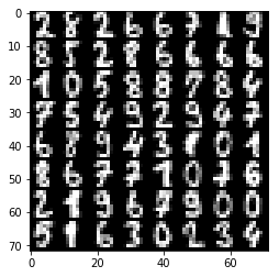
ミニバッチは次のようになります。img と label は numpy.ndarray として得られます。
img, label = data.next()
plt.imshow(tile_images(img), **imshow_opt)
print("labels: {}".format(label.reshape(8, 8)))
print("Label shape: {}".format(label.shape))
labels: [[ 2.  8.  2.  6.  6.  7.  1.  9.]
 [ 8.  5.  2.  8.  6.  6.  6.  6.]
 [ 1.  0.  5.  8.  8.  7.  8.  4.]
 [ 7.  5.  4.  9.  2.  9.  4.  7.]
 [ 6.  8.  9.  4.  3.  1.  0.  1.]
 [ 8.  6.  7.  7.  1.  0.  7.  6.]
 [ 2.  1.  9.  6.  7.  9.  0.  0.]
 [ 5.  1.  6.  3.  0.  2.  3.  4.]]
Label shape: (64, 1)
計算グラフの準備
NNabla では 誤差逆伝播法を用いる勾配降下法の最適化について 2 つの手法を提供しています。1 つは静的グラフで、もう 1 つは動的グラフによるものです。初めに、静的な方から見ていきましょう。
# Forward pass
x = nn.Variable(img.shape)  # Define an image variable
with nn.parameter_scope("affine1"):
    y = PF.affine(x, 10)  # Output is 10 class
このコードブロックは NNabla のグラフ作成機能の中で最も重要な特徴の 1 つである パラメータスコープの使い方 を示しています。1 行目で入力変数 x を定義します。2 行目で パラメータスコープ を作成します。 そして、3 行目で x に対してaffine変換 PF.affine を適用して、その結果を保持する変数 y を作ります。ここで、 PF ( parametric_function ) モジュールは ( 重みを含む ) affine変換、( カーネルを含む ) 畳み込み、( スケール因子など ) バッチ正規化のような、学習によって更新したいパラメータを含む関数を提供します。これらの関数を パラメトリック関数 といいます。 パラメータは関数呼び出しで作られ、ランダムに初期化され、 parameter_scope コンテキストを使って "affine1" という名前で登録されます。
# Building a loss graph
t = nn.Variable(label.shape)  # Define an target variable
loss = F.mean(F.softmax_cross_entropy(y, t))  # Softmax Xentropy fits multi-class classification problems
上記の残りの行では、目的関数を定義して、グラフの終端にロス関数を追加しています。静的グラフを構築しても、定義した計算は実際には実行されませんが、出力変数の状態は推測されることに注意してください。したがって、この時にそれぞれの変数の状態を調べることができます。
print("Printing shapes of variables")
print(x.shape)
print(y.shape)
print(t.shape)
print(loss.shape)  # empty tuple means scalar
Printing shapes of variables
(64, 1, 8, 8)
(64, 10)
(64, 1)
()
静的グラフの実行
グラフの終端である変数にある forward() メソッドを呼び出すことによって、グラフで定義された計算を実行することができます。入力は .d アクセサによってセットすることができます。このアクセサは numpy.ndarray として CPU から配列を受け取ります。
# Set data
x.d = img
t.d = label
# Execute a forward pass
loss.forward()
# Showing results
print("Prediction score of 0-th image: {}".format(y.d[0]))
print("Loss: {}".format(loss.d))
Prediction score of 0-th image: [  9.75851917   6.49118519  16.47323608  -1.36296904  -0.78583491
   4.08872032   7.84134388   2.42956853   3.31485462   3.61868763]
Loss: 10.6016616821
ネットワークはランダムに初期化されるので、この時点では出力は意味をなしません。
グラフによるバックプロパゲーション
parameter_scope に登録されることによって管理されるパラメータはディクショナリとして get_parameters() によってクエリできます。
print(nn.get_parameters())
OrderedDict([('affine1/affine/W', <Variable((64, 10), need_grad=True) at 0x7fa0ba361d50>), ('affine1/affine/b', <Variable((10,), need_grad=True) at 0x7fa0ba361ce8>)])
バックプロパゲーションを実行する前に、すべてのパラメータの勾配をゼロに初期化しておきます。
for param in nn.get_parameters().values():
    param.grad.zero()
そうすると、グラフの終端の変数で backward() メソッドを呼び出すことでバックプロパゲーションを実行することができます。
# Compute backward
loss.backward()
# Showing gradients.
for name, param in nn.get_parameters().items():
    print(name, param.shape, param.g.flat[:20])  # Showing first 20.
affine1/affine/W (64, 10) [  0.00000000e+00   0.00000000e+00   0.00000000e+00   0.00000000e+00
   0.00000000e+00   0.00000000e+00   0.00000000e+00   0.00000000e+00
   0.00000000e+00   0.00000000e+00   4.98418584e-02   8.72317329e-03
  -4.06671129e-02  -4.68742661e-02   2.52632981e-09   7.86017510e-04
   9.06870365e-02  -1.56249944e-02  -1.56217301e-02  -3.12499963e-02]
affine1/affine/b (10,) [ 0.42710391 -0.01852455  0.07369987 -0.04687012 -0.07798236 -0.03664626
  0.01651323 -0.1249291  -0.11862005 -0.09374455]
勾配は Variable の grad フィールドに格納されます。 .g アクセサは numpy.ndarray フォーマットで grad フィールドにアクセスするために使うことができます。
パラメータの最適化 ( = ニューラルネットワークの学習 )
パラメータを最適化するために、( ここでは S と名付けられた ) solver モジュールを用意しています。solver モジュールには、SGD 、モメンタム項をもつ SGD 、 Adam など、たくさんの最適化手法の実装が含まれています。以下のブロックは SGD solver を作り、ロジスティック回帰に用いるパラメータをそれにセットします。
# Create a solver (gradient-based optimizer)
learning_rate = 1e-3
solver = S.Sgd(learning_rate)
solver.set_parameters(nn.get_parameters())  # Set parameter variables to be updated.
次のブロックでは、最適化ループの 中で行われる 1 回分のステップを示しています。solver.zero_grad() は、上記で示したようにすべてのパラメータに対して .grad.zero() を呼び出すことと同じです。 バックプロパゲーションを実行したあとで、SGD solver クラスで実装されている重み減衰 ( Weight Decay ) を適用しています。そして最後に、勾配降下法によってパラメータを更新します。数式としては以下のようになります。
このとき \(\eta\) は学習率を表しています。
# One step of training
x.d, t.d = data.next()
loss.forward()
solver.zero_grad()  # Initialize gradients of all parameters to zero.
loss.backward()
solver.weight_decay(1e-5)  # Applying weight decay as an regularization
solver.update()
print(loss.d)
12.9438686371
次のブロックは最適化ステップをループによって繰り返しています。これによりロスが減少していくのが分かります。
for i in range(1000):
    x.d, t.d = data.next()
    loss.forward()
    solver.zero_grad()  # Initialize gradients of all parameters to zero.
    loss.backward()
    solver.weight_decay(1e-5)  # Applying weight decay as an regularization
    solver.update()
    if i % 100 == 0:  # Print for each 10 iterations
        print(i, loss.d)
0 12.6905069351
100 3.17041015625
200 1.60036706924
300 0.673069953918
400 0.951370298862
500 0.724424362183
600 0.361597299576
700 0.588107347488
800 0.28792989254
900 0.415006935596
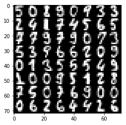
予測
次のコードは学習の結果を示しています。
x.d, t.d = data.next()  # Here we predict images from training set although it's useless.
y.forward()  # You can execute a sub graph.
plt.imshow(tile_images(x.d), **imshow_opt)
print("prediction:")
print(y.d.argmax(axis=1).reshape(8, 8))  # Taking a class index based on prediction score.
prediction:
[[5 0 1 9 0 1 3 3]
 [2 4 1 7 4 5 6 5]
 [7 7 9 7 9 0 7 3]
 [5 3 7 6 6 8 0 9]
 [0 1 3 5 5 5 4 9]
 [1 0 0 8 5 1 8 8]
 [7 5 0 7 6 9 0 0]
 [0 6 2 6 4 4 2 6]]
動的グラフのサポート
これは NNabla で計算グラフを実行するもう一つの方法です。この例では動的グラフの有用性を示しきれていませんが、その片鱗を伝えることができればと思います。
次のブロックでは、後に使うために計算グラフを構築するための関数を定義しています。
def logreg_forward(x):
    with nn.parameter_scope("affine1"):
        y = PF.affine(x, 10)
    return y

def logreg_loss(y, t):
    loss = F.mean(F.softmax_cross_entropy(y, t))  # Softmax Xentropy fits multi-class classification problems
    return loss
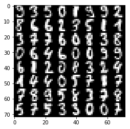
計算グラフの作成と同時にそのグラフで定義された計算を実行するためには、下記のブロックで示すように nnabla.auto_forward() コンテキストを使う必要があります。これにより、グラフ内で各演算を行う関数が呼び出された瞬間にその演算が実行されます。 ( また、グローバルで auto-forward 状態にするために nnabla.set_auto_forward(auto) を使うこともできます。 )
x = nn.Variable(img.shape)
t = nn.Variable(label.shape)
x.d, t.d = data.next()
with nn.auto_forward():  # Graph are executed
    y = logreg_forward(x)
    loss = logreg_loss(y, t)
print("Loss: {}".format(loss.d))
plt.imshow(tile_images(x.d), **imshow_opt)
print("prediction:")
print(y.d.argmax(axis=1).reshape(8, 8))
Loss: 0.43071603775
prediction:
[[9 3 5 0 1 9 9 2]
 [5 6 6 2 7 5 1 1]
 [3 7 7 6 0 8 3 8]
 [0 6 4 6 0 6 9 9]
 [6 1 2 5 8 3 2 4]
 [1 4 4 0 5 7 1 7]
 [7 8 9 5 8 3 7 8]
 [5 7 5 3 3 0 0 7]]
バックプロパゲーションは動的に作られたグラフでも実行できます。
solver.zero_grad()
loss.backward()
多層パーセプトロン ( MLP )
このセクションでは、多層パーセプトロン ( MLP ) を表す計算グラフの構築、およびその学習を行う例を見ていきます。
始める前に、ロジスティック回帰のサンプルで登録したすべてのパラメータを消去します。
nn.clear_parameters() # Clear all parameters
10 クラスの分類問題を解くために、任意の深さと幅をもつ MLP を構築する関数を定義します。
def mlp(x, hidden=[16, 32, 16]):
    hs = []
    with nn.parameter_scope("mlp"):  # Parameter scope can be nested
        h = x
        for hid, hsize in enumerate(hidden):
            with nn.parameter_scope("affine{}".format(hid + 1)):
                h = F.tanh(PF.affine(h, hsize))
                hs.append(h)
        with nn.parameter_scope("classifier"):
            y = PF.affine(h, 10)
    return y, hs
# Construct a MLP graph
y, hs = mlp(x)
print("Printing shapes")
print("x: {}".format(x.shape))
for i, h in enumerate(hs):
    print("h{}:".format(i + 1), h.shape)
print("y: {}".format(y.shape))
Printing shapes
x: (64, 1, 8, 8)
h1: (64, 16)
h2: (64, 32)
h3: (64, 16)
y: (64, 10)
# Training
loss = logreg_loss(y, t)  # Reuse logreg loss function.

# Copied from the above logreg example.
def training(steps, learning_rate):
    solver = S.Sgd(learning_rate)
    solver.set_parameters(nn.get_parameters())  # Set parameter variables to be updated.
    for i in range(steps):
        x.d, t.d = data.next()
        loss.forward()
        solver.zero_grad()  # Initialize gradients of all parameters to zero.
        loss.backward()
        solver.weight_decay(1e-5)  # Applying weight decay as an regularization
        solver.update()
        if i % 100 == 0:  # Print for each 10 iterations
            print(i, loss.d)


# Training
training(1000, 1e-2)
0 2.42193937302
100 1.83251476288
200 1.49943637848
300 1.30751883984
400 1.00974023342
500 0.904026031494
600 0.873289525509
700 0.725554704666
800 0.614291608334
900 0.555113613605
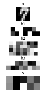
# Showing responses for each layer
num_plot = len(hs) + 2
gid = 1

def scale01(h):
    return (h - h.min()) / (h.max() - h.min())

def imshow(img, title):
    global gid
    plt.subplot(num_plot, 1, gid)
    gid += 1
    plt.title(title)
    plt.imshow(img, **imshow_opt)
    plt.axis('off')

plt.figure(figsize=(2, 5))
imshow(x.d[0, 0], 'x')
for hid, h in enumerate(hs):
    imshow(scale01(h.d[0]).reshape(-1, 8), 'h{}'.format(hid + 1))
imshow(scale01(y.d[0]).reshape(2, 5), 'y')
CUDA による高速な畳み込みニューラルネットワークの実行
ここでは、 CUDA を利用できる GPU を用いた CNN の高速な実行例を見ていきます。
nn.clear_parameters()
def cnn(x):
    with nn.parameter_scope("cnn"):  # Parameter scope can be nested
        with nn.parameter_scope("conv1"):
            c1 = F.tanh(PF.batch_normalization(
                PF.convolution(x, 4, (3, 3), pad=(1, 1), stride=(2, 2))))
        with nn.parameter_scope("conv2"):
            c2 = F.tanh(PF.batch_normalization(
                PF.convolution(c1, 8, (3, 3), pad=(1, 1))))
            c2 = F.average_pooling(c2, (2, 2))
        with nn.parameter_scope("fc3"):
            fc3 = F.tanh(PF.affine(c2, 32))
        with nn.parameter_scope("classifier"):
            y = PF.affine(fc3, 10)
    return y, [c1, c2, fc3]
NNabla で CUDA を利用するためには、まず、 nnabla-ext-cuda パッケージをインストールする必要があります。 インストールガイド を参照してください。CUDA エクステンションをインストールしたあと、グラフを作成する前にコンテキストを指定することによって、簡単に CUDA での実行に切り替えることができます。 cuDNN コンテキストは計算の高速実行が可能であることから、使用を強く推奨します。 コンテキストのクラスは nn.Context() によってインスタンス化できますが、コンテキストの記述子を指定することはユーザーにとって少し複雑かもしれません。そこで、 nnabla.ext_utils モジュールにある helper 関数 get_extension_context() を使ってコンテキストを作ることを推奨します。 NNabla は最初の引数 ( 拡張名 ) に渡されるコンテキストの指示子として cpu や cudnn を公式にサポートしています。
注 : cuDNN コンテキストを全体的なデフォルトのコンテキストとしてセットすることによって、作成された関数や solver は cuDNN モード (より好ましい ) でインスタンスが作られます。また、 nn.context_scope() を使うことでコンテキストを指定することができます。詳細は API リファレンス を参照してください。
# Run on CUDA
from nnabla.ext_utils import get_extension_context
cuda_device_id = 0
ctx = get_extension_context('cudnn', device_id=cuda_device_id)
print("Context: {}".format(ctx))
nn.set_default_context(ctx)  # Set CUDA as a default context.
y, hs = cnn(x)
loss = logreg_loss(y, t)
2017-06-26 23:09:54,555 [nnabla][INFO]: Initializing CUDA extension...
2017-06-26 23:09:54,731 [nnabla][INFO]: Initializing cuDNN extension...
Context: Context(backend='cpu|cuda', array_class='CudaCachedArray', device_id='0', compute_backend='default|cudnn')
training(1000, 1e-1)
0 2.34862923622
100 1.00527024269
200 0.416576713324
300 0.240603536367
400 0.254562884569
500 0.206138283014
600 0.220851421356
700 0.161689639091
800 0.230873346329
900 0.121101222932
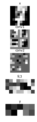
# Showing responses for each layer
num_plot = len(hs) + 2
gid = 1
plt.figure(figsize=(2, 8))
imshow(x.d[0, 0], 'x')
imshow(tile_images(hs[0].d[0][:, None]), 'conv1')
imshow(tile_images(hs[1].d[0][:, None]), 'conv2')
imshow(hs[2].d[0].reshape(-1, 8), 'fc3')
imshow(scale01(y.d[0]).reshape(2, 5), 'y')
nn.save_parameters は HDF5 フォーマットで parameter_scope に登録されたパラメータを書き出します。それは後述のサンプルで使用します。
path_cnn_params = "tmp.params.cnn.h5"
nn.save_parameters(path_cnn_params)
2017-06-26 23:09:56,132 [nnabla][INFO]: Parameter save (hdf5): tmp.params.cnn.h5
回帰型ニューラルネットワーク ( Elman RNN )
これは回帰型ニューラルネットワークの学習のサンプルです。
nn.clear_parameters()
def rnn(xs, h0, hidden=32):
    hs = []
    with nn.parameter_scope("rnn"):
        h = h0
        # Time step loop
        for x in xs:
            # Note: Parameter scopes are reused over time
            # which means parameters are shared over time.
            with nn.parameter_scope("x2h"):
                x2h = PF.affine(x, hidden, with_bias=False)
            with nn.parameter_scope("h2h"):
                h2h = PF.affine(h, hidden)
            h = F.tanh(x2h + h2h)
            hs.append(h)
        with nn.parameter_scope("classifier"):
            y = PF.affine(h, 10)
    return y, hs
この操作には特に意味はなく、デモを意図しています。画像を 2 × 2 のグリッドに分けて、それらを連続的に RNN に与えます。
def split_grid4(x):
    x0 = x[..., :4, :4]
    x1 = x[..., :4, 4:]
    x2 = x[..., 4:, :4]
    x3 = x[..., 4:, 4:]
    return x0, x1, x2, x3
hidden = 32
seq_img = split_grid4(img)
seq_x = [nn.Variable(subimg.shape) for subimg in seq_img]
h0 = nn.Variable((img.shape[0], hidden))  # Initial hidden state.
y, hs = rnn(seq_x, h0, hidden)
loss = logreg_loss(y, t)
# Copied from the above logreg example.
def training_rnn(steps, learning_rate):
    solver = S.Sgd(learning_rate)
    solver.set_parameters(nn.get_parameters())  # Set parameter variables to be updated.
    for i in range(steps):
        minibatch = data.next()
        img, t.d = minibatch
        seq_img = split_grid4(img)
        h0.d = 0  # Initialize as 0
        for x, subimg in zip(seq_x, seq_img):
            x.d = subimg
        loss.forward()
        solver.zero_grad()  # Initialize gradients of all parameters to zero.
        loss.backward()
        solver.weight_decay(1e-5)  # Applying weight decay as an regularization
        solver.update()
        if i % 100 == 0:  # Print for each 10 iterations
            print(i, loss.d)

training_rnn(1000, 1e-1)
0 2.62527275085
100 0.780260562897
200 0.486522495747
300 0.289345681667
400 0.249717146158
500 0.538961410522
600 0.276877015829
700 0.159639537334
800 0.249660402536
900 0.0925596579909
# Showing responses for each layer
num_plot = len(hs) + 2
gid = 1
plt.figure(figsize=(2, 8))
imshow(x.d[0, 0], 'x')
for hid, h in enumerate(hs):
    imshow(scale01(h.d[0]).reshape(-1, 8), 'h{}'.format(hid + 1))
imshow(scale01(y.d[0]).reshape(2, 5), 'y')

シャムネットワーク
このサンプルは、深層学習を使って 2 次元に、画像を分類別のデータセットに埋め込む方法を示しています。また、事前に学習されたネットワークを再利用する方法も説明しています。
初めに、 CNN のサンプルで学習されたパラメータをロードします。
nn.clear_parameters()
# Loading CNN pretrained parameters.
_ = nn.load_parameters(path_cnn_params)
2017-06-26 23:09:57,838 [nnabla][INFO]: Parameter load (<built-in function format>): tmp.params.cnn.h5
埋め込み関数を定義します。ネットワーク構造やパラメータの階層は以前の CNN のサンプルと同じであることに注意してください。これにより、保存したパラメータを再利用したり、パラメータをファインチューンしたりすることができます。
def cnn_embed(x, test=False):
    # Note: Identical configuration with the CNN example above.
    # Parameters pretrained in the above CNN example are used.
    with nn.parameter_scope("cnn"):
        with nn.parameter_scope("conv1"):
            c1 = F.tanh(PF.batch_normalization(PF.convolution(x, 4, (3, 3), pad=(1, 1), stride=(2, 2)), batch_stat=not test))
        with nn.parameter_scope("conv2"):
            c2 = F.tanh(PF.batch_normalization(PF.convolution(c1, 8, (3, 3), pad=(1, 1)), batch_stat=not test))
            c2 = F.average_pooling(c2, (2, 2))
        with nn.parameter_scope("fc3"):
            fc3 = PF.affine(c2, 32)
    # Additional affine for map into 2D.
    with nn.parameter_scope("embed2d"):
        embed = PF.affine(c2, 2)
    return embed, [c1, c2, fc3]

def siamese_loss(e0, e1, t, margin=1.0, eps=1e-4):
    dist = F.sum(F.squared_error(e0, e1), axis=1)  # Squared distance
    # Contrastive loss
    sim_cost = t * dist
    dissim_cost = (1 - t) * \
        (F.maximum_scalar(margin - (dist + eps) ** (0.5), 0) ** 2)
    return F.mean(sim_cost + dissim_cost)
2 つの CNN を作成し、上記で定義したコントラスティブロス関数で 2 つの CNN の出力を比較します。ここで、両方の CNN が同じパラメータの階層構造を有していることに注意してください。これはすなわち、両方のネットワークは利用するパラメータを共有しているということを意味します。
x0 = nn.Variable(img.shape)
x1 = nn.Variable(img.shape)
t = nn.Variable((img.shape[0],))  # Same class or not
e0, hs0 = cnn_embed(x0)
e1, hs1 = cnn_embed(x1)  # NOTE: parameters are shared
loss = siamese_loss(e0, e1, t)
def training_siamese(steps):
    for i in range(steps):
        minibatchs = []
        for _ in range(2):
            minibatch = data.next()
            minibatchs.append((minibatch[0].copy(), minibatch[1].copy()))
        x0.d, label0 = minibatchs[0]
        x1.d, label1 = minibatchs[1]
        t.d = (label0 == label1).astype(np.int).flat
        loss.forward()
        solver.zero_grad()  # Initialize gradients of all parameters to zero.
        loss.backward()
        solver.weight_decay(1e-5)  # Applying weight decay as an regularization
        solver.update()
        if i % 100 == 0:  # Print for each 10 iterations
            print(i, loss.d)
learning_rate = 1e-2
solver = S.Sgd(learning_rate)
with nn.parameter_scope("embed2d"):
    # Only 2d embedding affine will be updated.
    solver.set_parameters(nn.get_parameters())
training_siamese(2000)
# Decay learning rate
solver.set_learning_rate(solver.learning_rate() * 0.1)
training_siamese(2000)
0 0.150528043509
100 0.186870157719
200 0.149316266179
300 0.207163512707
400 0.171384960413
500 0.190256178379
600 0.138507723808
700 0.0918073058128
800 0.159692272544
900 0.0833697617054
1000 0.0839115008712
1100 0.104669973254
1200 0.0776312947273
1300 0.114788673818
1400 0.120309025049
1500 0.107732802629
1600 0.070114441216
1700 0.101728007197
1800 0.114350572228
1900 0.118794307113
0 0.0669310241938
100 0.0553173273802
200 0.0829797014594
300 0.0951051414013
400 0.128303915262
500 0.102963000536
600 0.0910559669137
700 0.0898950695992
800 0.119949311018
900 0.0603067912161
1000 0.105748720467
1100 0.108760476112
1200 0.0820947736502
1300 0.0971114039421
1400 0.0836166366935
1500 0.0899554267526
1600 0.109069615602
1700 0.0921652168036
1800 0.0759357959032
1900 0.100669950247
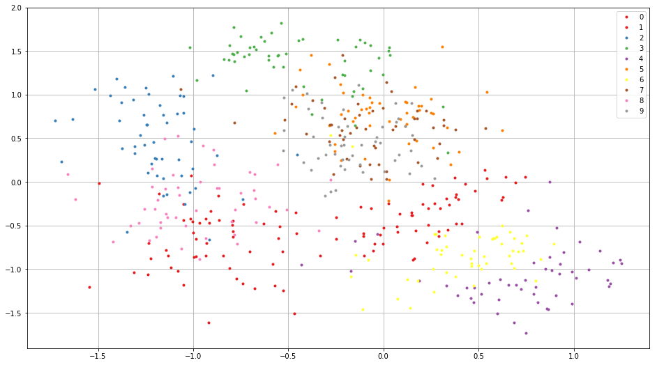
学習に用いた画像の埋め込みの結果を可視化してみましょう。同一クラスに属する画像は互いに近くに埋め込まれていることが分かります。
all_image = digits.images[:512, None]
all_label = digits.target[:512]
x_all = nn.Variable(all_image.shape)
x_all.d = all_image
with nn.auto_forward():
    embed, _ = cnn_embed(x_all, test=True)
plt.figure(figsize=(16, 9))
for i in range(10):
    c = plt.cm.Set1(i / 10.)  # Maybe it doesn't work in an older version of Matplotlib where color map lies in [0, 256)
    plt.plot(embed.d[all_label == i, 0].flatten(), embed.d[
             all_label == i, 1].flatten(), '.', c=c)
plt.legend(map(str, range(10)))
plt.grid()
付録
A. ロジスティック回帰
ここでは、最も簡単なニューラルネットワークであるロジスティック回帰 ( 1 層のパーセプトロン ) の学習の方法を説明します。ロジスティック回帰は線形分類問題 \(f : {\cal R}^{D\times 1} \rightarrow {\cal R}^{K\times 1}\)
で、 \(\mathbf x \in {\cal R}^{D \times 1}\) はベクトルへ平坦化された入力画像、 \(t \in \{0, 1, \cdots, K\}\) は目標ラベル、 \(\mathbf W \in {\cal R}^{K \times D}\) は重み行列、 \(\mathbf b \in {\cal R}^{K \times 1}\) はバイアスベクトル、 \(\mathbf \Theta \equiv \left\{\mathbf W, \mathbf b\right\}\) です。 Loss 関数は
のように定義されます。ここで、 \(\mathbf X \equiv \left\{\mathbf x_1, t_1, \cdots, \mathbf x_N, t_N\right\}\) はネットワークが学習に用いるデータセットを表し、 \(\sigma(\mathbf z)\) は \(\frac{\exp(-\mathbf z)}{\sum_{z \subset \mathbf z} \exp(-z)}\) のように定義されたソフトマックス演算で、 \(\left[\mathbf z\right]_i\) は \(\mathbf z\) の i 番目の要素を表しています。