NNabla Python API Demonstration Tutorial
Let us import nnabla first, and some additional useful tools.
# python2/3 compatibility
from __future__ import print_function
from __future__ import absolute_import
from __future__ import division
import nnabla as nn  # Abbreviate as nn for convenience.

import numpy as np
%matplotlib inline
import matplotlib.pyplot as plt
2017-09-27 14:00:30,785 [nnabla][INFO]: Initializing CPU extension...
NdArray
NdArray is a data container of a multi-dimensional array. NdArray is
device (e.g. CPU, CUDA) and type (e.g. uint8, float32) agnostic, in
which both type and device are implicitly cast or transferred when it
is used. Below, you create a NdArray with a shape of (2, 3, 4).
a = nn.NdArray((2, 3, 4))
You can see the values held inside a by the following. The values
are not initialized, and are created as float32 by default.
print(a.data)
[[[  9.42546995e+24   4.56809286e-41   8.47690058e-38   0.00000000e+00]
  [  7.38056336e+34   7.50334969e+28   1.17078231e-32   7.58387310e+31]
  [  7.87001454e-12   9.84394250e-12   6.85712044e+22   1.81785692e+31]]

 [[  1.84681296e+25   1.84933247e+20   4.85656319e+33   2.06176836e-19]
  [  6.80020530e+22   1.69307638e+22   2.11235872e-19   1.94316151e-19]
  [  1.81805047e+31   3.01289097e+29   2.07004908e-19   1.84648795e+25]]]
The accessor .data returns a reference to the values of NdArray as
numpy.ndarray. You can modify these by using the NumPy API as
follows.
print('[Substituting random values]')
a.data = np.random.randn(*a.shape)
print(a.data)
print('[Slicing]')
a.data[0, :, ::2] = 0
print(a.data)
[Substituting random values]
[[[ 0.36133638  0.22121875 -1.5912329  -0.33490974]
  [ 1.35962474  0.2165522   0.54483992 -0.61813235]
  [-0.13718799 -0.44104072 -0.51307833  0.73900551]]

 [[-0.59464753 -2.17738533 -0.28626776 -0.45654735]
  [ 0.73566747  0.87292582 -0.41605178  0.04792296]
  [-0.63856047  0.31966645 -0.63974309 -0.61385244]]]
[Slicing]
[[[ 0.          0.22121875  0.         -0.33490974]
  [ 0.          0.2165522   0.         -0.61813235]
  [ 0.         -0.44104072  0.          0.73900551]]

 [[-0.59464753 -2.17738533 -0.28626776 -0.45654735]
  [ 0.73566747  0.87292582 -0.41605178  0.04792296]
  [-0.63856047  0.31966645 -0.63974309 -0.61385244]]]
Note that the above operation is all done in the host device (CPU).
NdArray provides more efficient functions in case you want to fill all
values with a constant, .zero and .fill. They are lazily
evaluated when the data is requested (when neural network computation
requests the data, or when NumPy array is requested by Python) The
filling operation is executed within a specific device (e.g. CUDA GPU),
and more efficient if you specify the device setting, which we explain
later.
a.fill(1)  # Filling all values with one.
print(a.data)
[[[ 1.  1.  1.  1.]
  [ 1.  1.  1.  1.]
  [ 1.  1.  1.  1.]]

 [[ 1.  1.  1.  1.]
  [ 1.  1.  1.  1.]
  [ 1.  1.  1.  1.]]]
You can create an NdArray instance directly from a NumPy array object.
b = nn.NdArray.from_numpy_array(np.ones(a.shape))
print(b.data)
[[[ 1.  1.  1.  1.]
  [ 1.  1.  1.  1.]
  [ 1.  1.  1.  1.]]

 [[ 1.  1.  1.  1.]
  [ 1.  1.  1.  1.]
  [ 1.  1.  1.  1.]]]
NdArray is used in Variable class, as well as NNabla’s imperative computation of neural networks. We describe them in the later sections.
Variable
Variable class is used when you construct a neural network. The neural network can be described as a graph in which an edge represents a function (a.k.a operator and layer) which defines operation of a minimum unit of computation, and a node represents a variable which holds input/output values of a function (Function class is explained later). The graph is called “Computation Graph”.
In NNabla, a Variable, a node of a computation graph, holds two
NdArrays, one for storing the input or output values of a function
during forward propagation (executing computation graph in the forward
order), while another for storing the backward error signal (gradient)
during backward propagation (executing computation graph in backward
order to propagate error signals down to parameters (weights) of neural
networks). The first one is called data, the second is grad in
NNabla.
The following line creates a Variable instance with a shape of (2, 3,
4). It has data and grad as NdArray. The flag need_grad
is used to omit unnecessary gradient computation during backprop if set
to False.
x = nn.Variable([2, 3, 4], need_grad=True)
print('x.data:', x.data)
print('x.grad:', x.grad)
x.data: <NdArray((2, 3, 4)) at 0x7f575caf4ea0>
x.grad: <NdArray((2, 3, 4)) at 0x7f575caf4ea0>
You can get the shape by:
x.shape
(2, 3, 4)
Since both data and grad are NdArray, you can get a
reference to its values as NdArray with the .data accessor, but also
it can be referred by .d or .g property for data and grad
respectively.
print('x.data')
print(x.d)
x.d = 1.2345  # To avoid NaN
assert np.all(x.d == x.data.data), 'd: {} != {}'.format(x.d, x.data.data)
print('x.grad')
print(x.g)
x.g = 1.2345  # To avoid NaN
assert np.all(x.g == x.grad.data), 'g: {} != {}'.format(x.g, x.grad.data)

# Zeroing grad values
x.grad.zero()
print('x.grad (after `.zero()`)')
print(x.g)
x.data
[[[  9.42553452e+24   4.56809286e-41   8.32543479e-38   0.00000000e+00]
  [             nan              nan   0.00000000e+00   0.00000000e+00]
  [  3.70977305e+25   4.56809286e-41   3.78350585e-44   0.00000000e+00]]

 [[  5.68736600e-38   0.00000000e+00   1.86176378e-13   4.56809286e-41]
  [  4.74367616e+25   4.56809286e-41   5.43829710e+19   4.56809286e-41]
  [  0.00000000e+00   0.00000000e+00   2.93623372e-38   0.00000000e+00]]]
x.grad
[[[  9.42576510e+24   4.56809286e-41   9.42576510e+24   4.56809286e-41]
  [  9.27127763e-38   0.00000000e+00   9.27127763e-38   0.00000000e+00]
  [  1.69275966e+22   4.80112800e+30   1.21230330e+25   7.22962302e+31]]

 [[  1.10471027e-32   4.63080422e+27   2.44632805e+20   2.87606258e+20]
  [  4.46263300e+30   4.62311881e+30   7.65000750e+28   3.01339003e+29]
  [  2.08627352e-10   1.03961868e+21   7.99576678e+20   1.74441223e+22]]]
x.grad (after .zero())
[[[ 0.  0.  0.  0.]
  [ 0.  0.  0.  0.]
  [ 0.  0.  0.  0.]]

 [[ 0.  0.  0.  0.]
  [ 0.  0.  0.  0.]
  [ 0.  0.  0.  0.]]]
Like NdArray, a Variable can also be created from NumPy
array(s).
x2 = nn.Variable.from_numpy_array(np.ones((3,)), need_grad=True)
print(x2)
print(x2.d)
x3 = nn.Variable.from_numpy_array(np.ones((3,)), np.zeros((3,)), need_grad=True)
print(x3)
print(x3.d)
print(x3.g)
<Variable((3,), need_grad=True) at 0x7f572a5242c8>
[ 1.  1.  1.]
<Variable((3,), need_grad=True) at 0x7f572a5244a8>
[ 1.  1.  1.]
[ 0.  0.  0.]
Besides storing values of a computation graph, pointing a parent edge
(function) to trace the computation graph is an important role. Here
x doesn’t have any connection. Therefore, the .parent property
returns None.
print(x.parent)
None
Function
A function defines an operation block of a computation graph as we
described above. The module nnabla.functions offers various
functions (e.g. Convolution, Affine and ReLU). You can see the list of
functions available in the API reference
guide.
import nnabla.functions as F
As an example, here you will defines a computation graph that computes the element-wise Sigmoid function outputs for the input variable and sums up all values into a scalar. (This is simple enough to explain how it behaves but a meaningless example in the context of neural network training. We will show you a neural network example later.)
sigmoid_output = F.sigmoid(x)
sum_output = F.reduce_sum(sigmoid_output)
The function API in nnabla.functions takes one (or several)
Variable(s) and arguments (if any), and returns one (or several) output
Variable(s). The .parent points to the function instance which
created it. Note that no computation occurs at this time since we just
define the graph. (This is the default behavior of NNabla computation
graph API. You can also fire actual computation during graph definition
which we call “Dynamic mode” (explained later)).
print("sigmoid_output.parent.name:", sigmoid_output.parent.name)
print("x:", x)
print("sigmoid_output.parent.inputs refers to x:", sigmoid_output.parent.inputs)
sigmoid_output.parent.name: Sigmoid
x: <Variable((2, 3, 4), need_grad=True) at 0x7f572a51a778>
sigmoid_output.parent.inputs refers to x: [<Variable((2, 3, 4), need_grad=True) at 0x7f572a273a48>]
print("sum_output.parent.name:", sum_output.parent.name)
print("sigmoid_output:", sigmoid_output)
print("sum_output.parent.inputs refers to sigmoid_output:", sum_output.parent.inputs)
sum_output.parent.name: ReduceSum
sigmoid_output: <Variable((2, 3, 4), need_grad=True) at 0x7f572a524638>
sum_output.parent.inputs refers to sigmoid_output: [<Variable((2, 3, 4), need_grad=True) at 0x7f572a273a48>]
The .forward() at a leaf Variable executes the forward pass
computation in the computation graph.
sum_output.forward()
print("CG output:", sum_output.d)
print("Reference:", np.sum(1.0 / (1.0 + np.exp(-x.d))))
CG output: 18.59052085876465
Reference: 18.5905
The .backward() does the backward propagation through the graph.
Here we initialize the grad values as zero before backprop since the
NNabla backprop algorithm always accumulates the gradient in the root
variables.
x.grad.zero()
sum_output.backward()
print("d sum_o / d sigmoid_o:")
print(sigmoid_output.g)
print("d sum_o / d x:")
print(x.g)
d sum_o / d sigmoid_o:
[[[ 1.  1.  1.  1.]
  [ 1.  1.  1.  1.]
  [ 1.  1.  1.  1.]]

 [[ 1.  1.  1.  1.]
  [ 1.  1.  1.  1.]
  [ 1.  1.  1.  1.]]]
d sum_o / d x:
[[[ 0.17459197  0.17459197  0.17459197  0.17459197]
  [ 0.17459197  0.17459197  0.17459197  0.17459197]
  [ 0.17459197  0.17459197  0.17459197  0.17459197]]

 [[ 0.17459197  0.17459197  0.17459197  0.17459197]
  [ 0.17459197  0.17459197  0.17459197  0.17459197]
  [ 0.17459197  0.17459197  0.17459197  0.17459197]]]
NNabla is developed by mainly focused on neural network training and
inference. Neural networks have parameters to be learned associated with
computation blocks such as Convolution, Affine (a.k.a. fully connected,
dense etc.). In NNabla, the learnable parameters are also represented as
Variable objects. Just like input variables, those parameter
variables are also used by passing into Functions. For example,
Affine function takes input, weights and biases as inputs.
x = nn.Variable([5, 2])  # Input
w = nn.Variable([2, 3], need_grad=True)  # Weights
b = nn.Variable([3], need_grad=True)  # Biases
affine_out = F.affine(x, w, b)  # Create a graph including only affine
The above example takes an input with B=5 (batchsize) and D=2 (dimensions) and maps it to D’=3 outputs, i.e. (B, D’) output.
You may also notice that here you set need_grad=True only for
parameter variables (w and b). The x is a non-parameter variable and the
root of computation graph. Therefore, it doesn’t require gradient
computation. In this configuration, the gradient computation for x is
not executed in the first affine, which will omit the computation of
unnecessary backpropagation.
The next block sets data and initializes grad, then applies forward and backward computation.
# Set random input and parameters
x.d = np.random.randn(*x.shape)
w.d = np.random.randn(*w.shape)
b.d = np.random.randn(*b.shape)
# Initialize grad
x.grad.zero()  # Just for showing gradients are not computed when need_grad=False (default).
w.grad.zero()
b.grad.zero()

# Forward and backward
affine_out.forward()
affine_out.backward()
# Note: Calling backward at non-scalar Variable propagates 1 as error message from all element of outputs. .
You can see that affine_out holds an output of Affine.
print('F.affine')
print(affine_out.d)
print('Reference')
print(np.dot(x.d, w.d) + b.d)
F.affine
[[-0.17701732  2.86095762 -0.82298267]
 [-0.75544345 -1.16702223 -2.44841242]
 [-0.36278027 -3.4771595  -0.75681627]
 [ 0.32743117  0.24258983  1.30944324]
 [-0.87201929  1.94556415 -3.23357344]]
Reference
[[-0.1770173   2.86095762 -0.82298267]
 [-0.75544345 -1.16702223 -2.44841242]
 [-0.3627803  -3.4771595  -0.75681627]
 [ 0.32743117  0.24258983  1.309443  ]
 [-0.87201929  1.94556415 -3.23357344]]
The resulting gradients of weights and biases are as follows.
print("dw")
print(w.g)
print("db")
print(b.g)
dw
[[ 3.10820675  3.10820675  3.10820675]
 [ 0.37446201  0.37446201  0.37446201]]
db
[ 5.  5.  5.]
The gradient of x is not changed because need_grad is set as
False.
print(x.g)
[[ 0.  0.]
 [ 0.  0.]
 [ 0.  0.]
 [ 0.  0.]
 [ 0.  0.]]
Parametric Function
Considering parameters as inputs of Function enhances expressiveness
and flexibility of computation graphs. However, to define all parameters
for each learnable function is annoying for users to define a neural
network. In NNabla, trainable models are usually created by composing
functions that have optimizable parameters. These functions are called
“Parametric Functions”. The Parametric Function API provides various
parametric functions and an interface for composing trainable models.
To use parametric functions, import:
import nnabla.parametric_functions as PF
The function with optimizable parameter can be created as below.
with nn.parameter_scope("affine1"):
    c1 = PF.affine(x, 3)
The first line creates a parameter scope. The second line then
applies PF.affine - an affine transform - to x, and creates a
variable c1 holding that result. The parameters are created and
initialized randomly at function call, and registered by a name
“affine1” using parameter_scope context. The function
nnabla.get_parameters() allows to get the registered parameters.
nn.get_parameters()
OrderedDict([('affine1/affine/W',
              <Variable((2, 3), need_grad=True) at 0x7f572822f0e8>),
             ('affine1/affine/b',
              <Variable((3,), need_grad=True) at 0x7f572822f138>)])
The name= argument of any PF function creates the equivalent
parameter space to the above definition of PF.affine transformation
as below. It could save the space of your Python code. The
nnabla.parameter_scope is more useful when you group multiple
parametric functions such as Convolution-BatchNormalization found in a
typical unit of CNNs.
c1 = PF.affine(x, 3, name='affine1')
nn.get_parameters()
OrderedDict([('affine1/affine/W',
              <Variable((2, 3), need_grad=True) at 0x7f572822f0e8>),
             ('affine1/affine/b',
              <Variable((3,), need_grad=True) at 0x7f572822f138>)])
It is worth noting that the shapes of both outputs and parameter variables (as you can see above) are automatically determined by only providing the output size of affine transformation(in the example above the output size is 3). This helps to create a graph in an easy way.
c1.shape
(5, 3)
Parameter scope can be nested as follows (although a meaningless example).
with nn.parameter_scope('foo'):
    h = PF.affine(x, 3)
    with nn.parameter_scope('bar'):
        h = PF.affine(h, 4)
This creates the following.
nn.get_parameters()
OrderedDict([('affine1/affine/W',
              <Variable((2, 3), need_grad=True) at 0x7f572822f0e8>),
             ('affine1/affine/b',
              <Variable((3,), need_grad=True) at 0x7f572822f138>),
             ('foo/affine/W',
              <Variable((2, 3), need_grad=True) at 0x7f572822fa98>),
             ('foo/affine/b',
              <Variable((3,), need_grad=True) at 0x7f572822fae8>),
             ('foo/bar/affine/W',
              <Variable((3, 4), need_grad=True) at 0x7f572822f728>),
             ('foo/bar/affine/b',
              <Variable((4,), need_grad=True) at 0x7f572822fdb8>)])
Also, get_parameters() can be used in parameter_scope. For
example:
with nn.parameter_scope("foo"):
    print(nn.get_parameters())
OrderedDict([('affine/W', <Variable((2, 3), need_grad=True) at 0x7f572822fa98>), ('affine/b', <Variable((3,), need_grad=True) at 0x7f572822fae8>), ('bar/affine/W', <Variable((3, 4), need_grad=True) at 0x7f572822f728>), ('bar/affine/b', <Variable((4,), need_grad=True) at 0x7f572822fdb8>)])
nnabla.clear_parameters() can be used to delete registered
parameters under the scope.
with nn.parameter_scope("foo"):
    nn.clear_parameters()
print(nn.get_parameters())
OrderedDict([('affine1/affine/W', <Variable((2, 3), need_grad=True) at 0x7f572822f0e8>), ('affine1/affine/b', <Variable((3,), need_grad=True) at 0x7f572822f138>)])
MLP Example For Explanation
The following block creates a computation graph to predict one dimensional output from two dimensional inputs by a 2 layer fully connected neural network (multi-layer perceptron).
nn.clear_parameters()
batchsize = 16
x = nn.Variable([batchsize, 2])
with nn.parameter_scope("fc1"):
    h = F.tanh(PF.affine(x, 512))
with nn.parameter_scope("fc2"):
    y = PF.affine(h, 1)
print("Shapes:", h.shape, y.shape)
Shapes: (16, 512) (16, 1)
This will create the following parameter variables.
nn.get_parameters()
OrderedDict([('fc1/affine/W',
              <Variable((2, 512), need_grad=True) at 0x7f572822fef8>),
             ('fc1/affine/b',
              <Variable((512,), need_grad=True) at 0x7f572822f9a8>),
             ('fc2/affine/W',
              <Variable((512, 1), need_grad=True) at 0x7f572822f778>),
             ('fc2/affine/b',
              <Variable((1,), need_grad=True) at 0x7f572822ff98>)])
As described above, you can execute the forward pass by calling forward method at the terminal variable.
x.d = np.random.randn(*x.shape)  # Set random input
y.forward()
print(y.d)
[[-0.05708594]
 [ 0.01661986]
 [-0.34168088]
 [ 0.05822293]
 [-0.16566885]
 [-0.04867431]
 [ 0.2633169 ]
 [ 0.10496549]
 [-0.01291842]
 [-0.09726256]
 [-0.05720493]
 [-0.09691752]
 [-0.07822668]
 [-0.17180404]
 [ 0.11970415]
 [-0.08222144]]
Training a neural networks needs a loss value to be minimized by gradient descent with backprop. In NNabla, loss function is also a just function, and packaged in the functions module.
# Variable for label
label = nn.Variable([batchsize, 1])
# Set loss
loss = F.reduce_mean(F.squared_error(y, label))

# Execute forward pass.
label.d = np.random.randn(*label.shape)  # Randomly generate labels
loss.forward()
print(loss.d)
1.9382084608078003
As you’ve seen above, NNabla backward accumulates the gradients at
the root variables. You have to initialize the grad of the parameter
variables before backprop (We will show you the easiest way with
Solver API).
# Collect all parameter variables and init grad.
for name, param in nn.get_parameters().items():
    param.grad.zero()
# Gradients are accumulated to grad of params.
loss.backward()
Imperative Mode
After performing backprop, gradients are held in parameter variable grads. The next block will update the parameters with vanilla gradient descent.
for name, param in nn.get_parameters().items():
    param.data -= param.grad * 0.001  # 0.001 as learning rate
The above computation is an example of NNabla’s “Imperative Mode” for
executing neural networks. Normally, NNabla functions (instances of
nnabla.functions)
take Variables as their input. When at least one NdArray is
provided as an input for NNabla functions (instead of Variables),
the function computation will be fired immediately, and returns an
NdArray as the output, instead of returning a Variable. In the
above example, the NNabla functions F.mul_scalar and F.sub2 are
called by the overridden operators * and -=, respectively.
In other words, NNabla’s “Imperative mode” doesn’t create a computation graph, and can be used like NumPy. If device acceleration such as CUDA is enabled, it can be used like NumPy empowered with device acceleration. Parametric functions can also be used with NdArray input(s). The following block demonstrates a simple imperative execution example.
# A simple example of imperative mode.
xi = nn.NdArray.from_numpy_array(np.arange(4).reshape(2, 2))
yi = F.relu(xi - 1)
print(xi.data)
print(yi.data)
[[0 1]
 [2 3]]
[[ 0.  0.]
 [ 1.  2.]]
Note that in-place substitution from the rhs to the lhs cannot be done
by the = operator. For example, when x is an NdArray,
writing x = x + 1 will not increment all values of x -
instead, the expression on the rhs will create a new NdArray
object that is different from the one originally bound by x, and binds
the new NdArray object to the Python variable x on the lhs.
For in-place editing of NdArrays, the in-place assignment operators
+=, -=, *=, and /= can be used. The copy_from method
can also be used to copy values of an existing NdArray to another.
For example, increment 1 to x, an NdArray, can be done by
x.copy_from(x+1). The copy is performed with device acceleration if
a device context is specified by using nnabla.set_default_context or
nnabla.context_scope.
# The following doesn't perform substitution but assigns a new NdArray object to `xi`.
# xi = xi + 1

# The following copies the result of `xi + 1` to `xi`.
xi.copy_from(xi + 1)
assert np.all(xi.data == (np.arange(4).reshape(2, 2) + 1))

# Inplace operations like `+=`, `*=` can also be used (more efficient).
xi += 1
assert np.all(xi.data == (np.arange(4).reshape(2, 2) + 2))
Solver
NNabla provides stochastic gradient descent algorithms to optimize
parameters listed in the nnabla.solvers module. The parameter
updates demonstrated above can be replaced with this Solver API, which
is easier and usually faster.
from nnabla import solvers as S
solver = S.Sgd(lr=0.00001)
solver.set_parameters(nn.get_parameters())
# Set random data
x.d = np.random.randn(*x.shape)
label.d = np.random.randn(*label.shape)

# Forward
loss.forward()
Just call the the following solver method to fill zero grad region, then backprop
solver.zero_grad()
loss.backward()
The following block updates parameters with the Vanilla Sgd rule (equivalent to the imperative example above).
solver.update()
Toy Problem To Demonstrate Training
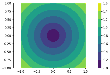
The following function defines a regression problem which computes the norm of a vector.
def vector2length(x):
    # x : [B, 2] where B is number of samples.
    return np.sqrt(np.sum(x ** 2, axis=1, keepdims=True))
We visualize this mapping with the contour plot by matplotlib as follows.
# Data for plotting contour on a grid data.
xs = np.linspace(-1, 1, 100)
ys = np.linspace(-1, 1, 100)
grid = np.meshgrid(xs, ys)
X = grid[0].flatten()
Y = grid[1].flatten()

def plot_true():
    """Plotting contour of true mapping from a grid data created above."""
    plt.contourf(xs, ys, vector2length(np.hstack([X[:, None], Y[:, None]])).reshape(100, 100))
    plt.axis('equal')
    plt.colorbar()

plot_true()
We define a deep prediction neural network.
def length_mlp(x):
    h = x
    for i, hnum in enumerate([4, 8, 4, 2]):
        h = F.tanh(PF.affine(h, hnum, name="fc{}".format(i)))
    y = PF.affine(h, 1, name='fc')
    return y
nn.clear_parameters()
batchsize = 100
x = nn.Variable([batchsize, 2])
y = length_mlp(x)
label = nn.Variable([batchsize, 1])
loss = F.reduce_mean(F.squared_error(y, label))
We created a 5 layers deep MLP using for-loop. Note that only 3 lines of the code potentially create infinitely deep neural networks. The next block adds helper functions to visualize the learned function.
def predict(inp):
    ret = []
    for i in range(0, inp.shape[0], x.shape[0]):
        xx = inp[i:i + x.shape[0]]
        # Imperative execution
        xi = nn.NdArray.from_numpy_array(xx)
        yi = length_mlp(xi)
        ret.append(yi.data.copy())
    return np.vstack(ret)

def plot_prediction():
    plt.contourf(xs, ys, predict(np.hstack([X[:, None], Y[:, None]])).reshape(100, 100))
    plt.colorbar()
    plt.axis('equal')
Next we instantiate a solver object as follows. We use Adam optimizer which is one of the most popular SGD algorithm used in the literature.
from nnabla import solvers as S
solver = S.Adam(alpha=0.01)
solver.set_parameters(nn.get_parameters())
The following function generates data from the true system infinitely.
def random_data_provider(n):
    x = np.random.uniform(-1, 1, size=(n, 2))
    y = vector2length(x)
    return x, y
In the next block, we run 2000 training steps (SGD updates).
num_iter = 2000
for i in range(num_iter):
    # Sample data and set them to input variables of training.
    xx, ll = random_data_provider(batchsize)
    x.d = xx
    label.d = ll
    # Forward propagation given inputs.
    loss.forward(clear_no_need_grad=True)
    # Parameter gradients initialization and gradients computation by backprop.
    solver.zero_grad()
    loss.backward(clear_buffer=True)
    # Apply weight decay and update by Adam rule.
    solver.weight_decay(1e-6)
    solver.update()
    # Just print progress.
    if i % 100 == 0 or i == num_iter - 1:
        print("Loss@{:4d}: {}".format(i, loss.d))
Loss@   0: 0.6976373195648193
Loss@ 100: 0.08075223118066788
Loss@ 200: 0.005213144235312939
Loss@ 300: 0.001955194864422083
Loss@ 400: 0.0011660841992124915
Loss@ 500: 0.0006421314901672304
Loss@ 600: 0.0009330055327154696
Loss@ 700: 0.0008817618945613503
Loss@ 800: 0.0006205961108207703
Loss@ 900: 0.0009072928223758936
Loss@1000: 0.0008160348515957594
Loss@1100: 0.0011569359339773655
Loss@1200: 0.000837412488181144
Loss@1300: 0.0011542742140591145
Loss@1400: 0.0005833200993947685
Loss@1500: 0.0009848927147686481
Loss@1600: 0.0005141657311469316
Loss@1700: 0.0009339841199107468
Loss@1800: 0.000950580753851682
Loss@1900: 0.0005430278833955526
Loss@1999: 0.0007046313839964569
Memory usage optimization: You may notice that, in the above
updates, .forward() is called with the clear_no_need_grad=
option, and .backward() is called with the clear_buffer= option.
Training of neural network in more realistic scenarios usually consumes
huge memory due to the nature of backpropagation algorithm, in which all
of the forward variable buffer data should be kept in order to
compute the gradient of a function. In a naive implementation, we keep
all the variable data and grad living until the NdArray
objects are not referenced (i.e. the graph is deleted). The clear_*
options in .forward() and .backward() enables to save memory
consumption due to that by clearing (erasing) memory of data and
grad when it is not referenced by any subsequent computation. (More
precisely speaking, it doesn’t free memory actually. We use our memory
pool engine by default to avoid memory alloc/free overhead). The
unused buffers can be re-used in subsequent computation. See the
document of Variable for more details. Note that the following
loss.forward(clear_buffer=True) clears data of any intermediate
variables. If you are interested in intermediate variables for some
purposes (e.g. debug, log), you can use the .persistent flag to
prevent clearing buffer of a specific Variable like below.
loss.forward(clear_buffer=True)
print("The prediction `y` is cleared because it's an intermediate variable.")
print(y.d.flatten()[:4])  # to save space show only 4 values
y.persistent = True
loss.forward(clear_buffer=True)
print("The prediction `y` is kept by the persistent flag.")
print(y.d.flatten()[:4])  # to save space show only 4 value
The predictionyis cleared because it's an intermediate variable. [ 2.27279830e-04 6.02164946e-05 5.33679675e-04 2.35557582e-05] The predictionyis kept by the persistent flag. [ 1.0851264 0.87657517 0.79603785 0.40098712]
We can confirm the prediction performs fairly well by looking at the following visualization of the ground truth and prediction function.
plt.subplot(121)
plt.title("Ground truth")
plot_true()
plt.subplot(122)
plt.title("Prediction")
plot_prediction()

You can save learned parameters by nnabla.save_parameters and load
by nnabla.load_parameters.
path_param = "param-vector2length.h5"
nn.save_parameters(path_param)
# Remove all once
nn.clear_parameters()
nn.get_parameters()
2017-09-27 14:00:40,544 [nnabla][INFO]: Parameter save (.h5): param-vector2length.h5
OrderedDict()
# Load again
nn.load_parameters(path_param)
print('\n'.join(map(str, nn.get_parameters().items())))
2017-09-27 14:00:40,564 [nnabla][INFO]: Parameter load (<built-in function format>): param-vector2length.h5
('fc0/affine/W', <Variable((2, 4), need_grad=True) at 0x7f576328df48>)
('fc0/affine/b', <Variable((4,), need_grad=True) at 0x7f57245f2868>)
('fc1/affine/W', <Variable((4, 8), need_grad=True) at 0x7f576328def8>)
('fc1/affine/b', <Variable((8,), need_grad=True) at 0x7f5727ee5c78>)
('fc2/affine/W', <Variable((8, 4), need_grad=True) at 0x7f5763297318>)
('fc2/affine/b', <Variable((4,), need_grad=True) at 0x7f5727d29908>)
('fc3/affine/W', <Variable((4, 2), need_grad=True) at 0x7f57632973b8>)
('fc3/affine/b', <Variable((2,), need_grad=True) at 0x7f57632974a8>)
('fc/affine/W', <Variable((2, 1), need_grad=True) at 0x7f57632974f8>)
('fc/affine/b', <Variable((1,), need_grad=True) at 0x7f5763297598>)
Both save and load functions can also be used in a parameter scope.
with nn.parameter_scope('foo'):
    nn.load_parameters(path_param)
print('\n'.join(map(str, nn.get_parameters().items())))
2017-09-27 14:00:40,714 [nnabla][INFO]: Parameter load (<built-in function format>): param-vector2length.h5
('fc0/affine/W', <Variable((2, 4), need_grad=True) at 0x7f576328df48>)
('fc0/affine/b', <Variable((4,), need_grad=True) at 0x7f57245f2868>)
('fc1/affine/W', <Variable((4, 8), need_grad=True) at 0x7f576328def8>)
('fc1/affine/b', <Variable((8,), need_grad=True) at 0x7f5727ee5c78>)
('fc2/affine/W', <Variable((8, 4), need_grad=True) at 0x7f5763297318>)
('fc2/affine/b', <Variable((4,), need_grad=True) at 0x7f5727d29908>)
('fc3/affine/W', <Variable((4, 2), need_grad=True) at 0x7f57632973b8>)
('fc3/affine/b', <Variable((2,), need_grad=True) at 0x7f57632974a8>)
('fc/affine/W', <Variable((2, 1), need_grad=True) at 0x7f57632974f8>)
('fc/affine/b', <Variable((1,), need_grad=True) at 0x7f5763297598>)
('foo/fc0/affine/W', <Variable((2, 4), need_grad=True) at 0x7f5763297958>)
('foo/fc0/affine/b', <Variable((4,), need_grad=True) at 0x7f57632978b8>)
('foo/fc1/affine/W', <Variable((4, 8), need_grad=True) at 0x7f572a51ac78>)
('foo/fc1/affine/b', <Variable((8,), need_grad=True) at 0x7f5763297c78>)
('foo/fc2/affine/W', <Variable((8, 4), need_grad=True) at 0x7f5763297a98>)
('foo/fc2/affine/b', <Variable((4,), need_grad=True) at 0x7f5763297d68>)
('foo/fc3/affine/W', <Variable((4, 2), need_grad=True) at 0x7f5763297e08>)
('foo/fc3/affine/b', <Variable((2,), need_grad=True) at 0x7f5763297ea8>)
('foo/fc/affine/W', <Variable((2, 1), need_grad=True) at 0x7f5763297f48>)
('foo/fc/affine/b', <Variable((1,), need_grad=True) at 0x7f5763297cc8>)
!rm {path_param} # Clean ups