NNabla by Examples

This tutorial demonstrates how you can write a script to train a neural network by using a simple hand digits classification task.

Note: This tutorial notebook requires scikit-learn and matplotlib installed in your Python environment.

First let us prepare some dependencies.

import nnabla as nn

import nnabla.functions as F
import nnabla.parametric_functions as PF
import nnabla.solvers as S
from nnabla.monitor import tile_images

import numpy as np
import matplotlib.pyplot as plt
import tiny_digits
%matplotlib inline

np.random.seed(0)
imshow_opt = dict(cmap='gray', interpolation='nearest')

2017-06-26 23:09:49,971 [nnabla][INFO]: Initializing CPU extension...

The tiny_digits module is located under this folder. It provides some utilities for loading a handwritten-digit classification dataset (MNIST) available in scikit-learn.

Logistic Regression

We will first start by defining a computation graph for logistic regression. (For details on logistic regression, see Appendix A.)

The training will be done by gradient descent, where gradients are calculated using the error backpropagation algorithm (backprop).

Preparing a Toy Dataset

This section just prepares a dataset to be used for demonstration of NNabla usage.

digits = tiny_digits.load_digits(n_class=10)
tiny_digits.plot_stats(digits)

Num images: 1797
Image shape: (8, 8)
Labels: [0 1 2 3 4 5 6 7 8 9]

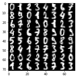
The next block creates a dataset loader which is a generator providing images and labels as minibatches. Note that this dataset is just an example purpose and not a part of NNabla.

data = tiny_digits.data_iterator_tiny_digits(digits, batch_size=64, shuffle=True)

2017-06-26 23:09:50,545 [nnabla][INFO]: DataSource with shuffle(True)
2017-06-26 23:09:50,546 [nnabla][INFO]: Using DataSourceWithMemoryCache
2017-06-26 23:09:50,546 [nnabla][INFO]: DataSource with shuffle(True)
2017-06-26 23:09:50,547 [nnabla][INFO]: On-memory
2017-06-26 23:09:50,547 [nnabla][INFO]: Using DataIterator

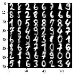
A minibatch is as follows. img and label are in numpy.ndarray.

img, label = data.next()
plt.imshow(tile_images(img), **imshow_opt)
print("labels: {}".format(label.reshape(8, 8)))
print("Label shape: {}".format(label.shape))

labels: [[ 2.  8.  2.  6.  6.  7.  1.  9.]
 [ 8.  5.  2.  8.  6.  6.  6.  6.]
 [ 1.  0.  5.  8.  8.  7.  8.  4.]
 [ 7.  5.  4.  9.  2.  9.  4.  7.]
 [ 6.  8.  9.  4.  3.  1.  0.  1.]
 [ 8.  6.  7.  7.  1.  0.  7.  6.]
 [ 2.  1.  9.  6.  7.  9.  0.  0.]
 [ 5.  1.  6.  3.  0.  2.  3.  4.]]
Label shape: (64, 1)

Preparing the Computation Graph

NNabla provides two different ways for backprop-based gradient descent optimization. One is with a static graph, and another is with a dynamic graph. We are going to show a static version first.

# Forward pass
x = nn.Variable(img.shape)  # Define an image variable
with nn.parameter_scope("affine1"):
    y = PF.affine(x, 10)  # Output is 10 class

This code block shows one of the most important features in graph building in NNabla, the parameter scope. The first line defines an input variable x. The second line creates a parameter scope. The third line then applies PF.affine - an affine transform - to x, and creates a variable y holding that result. Here, the PF (parametric_function) module provides functions that contain learnable parameters, such as affine transforms (which contains weights), convolution (which contains kernels) and batch normalization (which contains transformation factors and coefficients). We will call these functions as parametric functions. The parameters are created and initialized randomly at function call, and registered by a name “affine1” using parameter_scope context.

# Building a loss graph
t = nn.Variable(label.shape)  # Define an target variable
loss = F.mean(F.softmax_cross_entropy(y, t))  # Softmax Xentropy fits multi-class classification problems

The remaining lines shown above define a target variable and attach functions for loss at the end of the graph. Note that the static graph build doesn’t execute any computation, but the shapes of output variables are inferred. Therefore, we can inspect the shapes of each variable at this time:

print("Printing shapes of variables")
print(x.shape)
print(y.shape)
print(t.shape)
print(loss.shape)  # empty tuple means scalar

Printing shapes of variables
(64, 1, 8, 8)
(64, 10)
(64, 1)
()

Executing a static graph

You can execute the computation of the graph by calling the forward() method in a sink variable. Inputs can be set via .d accessor. It will borrow CPU array references as numpy.ndarray.

# Set data
x.d = img
t.d = label
# Execute a forward pass
loss.forward()
# Showing results
print("Prediction score of 0-th image: {}".format(y.d[0]))
print("Loss: {}".format(loss.d))

Prediction score of 0-th image: [  9.75851917   6.49118519  16.47323608  -1.36296904  -0.78583491
   4.08872032   7.84134388   2.42956853   3.31485462   3.61868763]
Loss: 10.6016616821

The output doesn’t make sense since the network is just randomly initialized.

Backward propagation through the graph

The parameters registered by parameter_scope management function can be queried by get_parameters() as a dict format.

print(nn.get_parameters())

OrderedDict([('affine1/affine/W', <Variable((64, 10), need_grad=True) at 0x7fa0ba361d50>), ('affine1/affine/b', <Variable((10,), need_grad=True) at 0x7fa0ba361ce8>)])

Before executing backpropagation, we should initialize gradient buffers of all parameter to zeros.

for param in nn.get_parameters().values():
    param.grad.zero()

Then, you can execute backprop by calling backward() method at the sink variable.

# Compute backward
loss.backward()
# Showing gradients.
for name, param in nn.get_parameters().items():
    print(name, param.shape, param.g.flat[:20])  # Showing first 20.

affine1/affine/W (64, 10) [  0.00000000e+00   0.00000000e+00   0.00000000e+00   0.00000000e+00
   0.00000000e+00   0.00000000e+00   0.00000000e+00   0.00000000e+00
   0.00000000e+00   0.00000000e+00   4.98418584e-02   8.72317329e-03
  -4.06671129e-02  -4.68742661e-02   2.52632981e-09   7.86017510e-04
   9.06870365e-02  -1.56249944e-02  -1.56217301e-02  -3.12499963e-02]
affine1/affine/b (10,) [ 0.42710391 -0.01852455  0.07369987 -0.04687012 -0.07798236 -0.03664626
  0.01651323 -0.1249291  -0.11862005 -0.09374455]

Gradient is stored in grad field of Variable. .g accessor can be used to access grad data in numpy.ndarray format.

Optimizing parameters (=Training)

To optimize parameters, we provide solver module (aliased as S here). The solver module contains a bunch of optimizer implementations such as SGD, SGD with momentum, Adam etc. The below block creates SGD solver and sets parameters of logistic regression to it.

# Create a solver (gradient-based optimizer)
learning_rate = 1e-3
solver = S.Sgd(learning_rate)
solver.set_parameters(nn.get_parameters())  # Set parameter variables to be updated.

In the next block, we demonstrate a single step of optimization loop. solver.zero_grad() line does equivalent to calling .grad.zero() for all parameters as we shown above. After backward computation, we apply weight decay, then applying gradient descent implemented in Sgd solver class as follows

\[\theta \leftarrow \theta - \eta \nabla_{\theta} L(\theta, X_{\mathrm minibatch})\]

where \(\eta\) denotes learning rate.

# One step of training
x.d, t.d = data.next()
loss.forward()
solver.zero_grad()  # Initialize gradients of all parameters to zero.
loss.backward()
solver.weight_decay(1e-5)  # Applying weight decay as an regularization
solver.update()
print(loss.d)

12.9438686371

Next block iterates optimization steps, and shows the loss decreases.

for i in range(1000):
    x.d, t.d = data.next()
    loss.forward()
    solver.zero_grad()  # Initialize gradients of all parameters to zero.
    loss.backward()
    solver.weight_decay(1e-5)  # Applying weight decay as an regularization
    solver.update()
    if i % 100 == 0:  # Print for each 10 iterations
        print(i, loss.d)

12.6905069351
3.17041015625
1.60036706924
0.673069953918
0.951370298862
0.724424362183
0.361597299576
0.588107347488
0.28792989254
0.415006935596

Show prediction

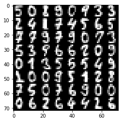
The following code displays training results.

x.d, t.d = data.next()  # Here we predict images from training set although it's useless.
y.forward()  # You can execute a sub graph.
plt.imshow(tile_images(x.d), **imshow_opt)
print("prediction:")
print(y.d.argmax(axis=1).reshape(8, 8))  # Taking a class index based on prediction score.

prediction:
[[5 0 1 9 0 1 3 3]
 [2 4 1 7 4 5 6 5]
 [7 7 9 7 9 0 7 3]
 [5 3 7 6 6 8 0 9]
 [0 1 3 5 5 5 4 9]
 [1 0 0 8 5 1 8 8]
 [7 5 0 7 6 9 0 0]
 [0 6 2 6 4 4 2 6]]

Dynamic graph construction support

This is another way of running computation graph in NNabla. This example doesn’t show how useful dynamic graph is, but shows a bit of flavor.

The next block just define computation graph building as functions for later use.

def logreg_forward(x):
    with nn.parameter_scope("affine1"):
        y = PF.affine(x, 10)
    return y

def logreg_loss(y, t):
    loss = F.mean(F.softmax_cross_entropy(y, t))  # Softmax Xentropy fits multi-class classification problems
    return loss

To run a computation graph dynamically during creation, you use nnabla.auto_forward() context as you see in the below block. By this, computation is fired immediately at functions are called. (You can also use nnabla.set_auto_forward(auto) to set the auto-forward state globally.)

x = nn.Variable(img.shape)
t = nn.Variable(label.shape)
x.d, t.d = data.next()
with nn.auto_forward():  # Graph are executed
    y = logreg_forward(x)
    loss = logreg_loss(y, t)
print("Loss: {}".format(loss.d))
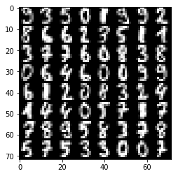
plt.imshow(tile_images(x.d), **imshow_opt)
print("prediction:")
print(y.d.argmax(axis=1).reshape(8, 8))

Loss: 0.43071603775
prediction:
[[9 3 5 0 1 9 9 2]
 [5 6 6 2 7 5 1 1]
 [3 7 7 6 0 8 3 8]
 [0 6 4 6 0 6 9 9]
 [6 1 2 5 8 3 2 4]
 [1 4 4 0 5 7 1 7]
 [7 8 9 5 8 3 7 8]
 [5 7 5 3 3 0 0 7]]

Backward computation can be done on a dynamically constructed graph.

solver.zero_grad()
loss.backward()

Multi-Layer Perceptron (MLP)

In this section, you see an example of MLP graph building and training.

Before starting, we clear all parameters registered in the logistic regression example.

nn.clear_parameters()  # Clear all parameters

Here is the function that builds a MLP with an arbitrary depth and width for 10 class classification.

def mlp(x, hidden=[16, 32, 16]):
    hs = []
    with nn.parameter_scope("mlp"):  # Parameter scope can be nested
        h = x
        for hid, hsize in enumerate(hidden):
            with nn.parameter_scope("affine{}".format(hid + 1)):
                h = F.tanh(PF.affine(h, hsize))
                hs.append(h)
        with nn.parameter_scope("classifier"):
            y = PF.affine(h, 10)
    return y, hs

# Construct a MLP graph
y, hs = mlp(x)

print("Printing shapes")
print("x: {}".format(x.shape))
for i, h in enumerate(hs):
    print("h{}:".format(i + 1), h.shape)
print("y: {}".format(y.shape))

Printing shapes
x: (64, 1, 8, 8)
h1: (64, 16)
h2: (64, 32)
h3: (64, 16)
y: (64, 10)

# Training
loss = logreg_loss(y, t)  # Reuse logreg loss function.

# Copied from the above logreg example.
def training(steps, learning_rate):
    solver = S.Sgd(learning_rate)
    solver.set_parameters(nn.get_parameters())  # Set parameter variables to be updated.
    for i in range(steps):
        x.d, t.d = data.next()
        loss.forward()
        solver.zero_grad()  # Initialize gradients of all parameters to zero.
        loss.backward()
        solver.weight_decay(1e-5)  # Applying weight decay as an regularization
        solver.update()
        if i % 100 == 0:  # Print for each 10 iterations
            print(i, loss.d)


# Training
training(1000, 1e-2)

2.42193937302
1.83251476288
1.49943637848
1.30751883984
1.00974023342
0.904026031494
0.873289525509
0.725554704666
0.614291608334
0.555113613605

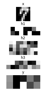
# Showing responses for each layer
num_plot = len(hs) + 2
gid = 1

def scale01(h):
    return (h - h.min()) / (h.max() - h.min())

def imshow(img, title):
    global gid
    plt.subplot(num_plot, 1, gid)
    gid += 1
    plt.title(title)
    plt.imshow(img, **imshow_opt)
    plt.axis('off')

plt.figure(figsize=(2, 5))
imshow(x.d[0, 0], 'x')
for hid, h in enumerate(hs):
    imshow(scale01(h.d[0]).reshape(-1, 8), 'h{}'.format(hid + 1))
imshow(scale01(y.d[0]).reshape(2, 5), 'y')

Convolutional Neural Network with CUDA acceleration

Here we demonstrates a CNN with CUDA GPU acceleration.

nn.clear_parameters()

def cnn(x):
    with nn.parameter_scope("cnn"):  # Parameter scope can be nested
        with nn.parameter_scope("conv1"):
            c1 = F.tanh(PF.batch_normalization(
                PF.convolution(x, 4, (3, 3), pad=(1, 1), stride=(2, 2))))
        with nn.parameter_scope("conv2"):
            c2 = F.tanh(PF.batch_normalization(
                PF.convolution(c1, 8, (3, 3), pad=(1, 1))))
            c2 = F.average_pooling(c2, (2, 2))
        with nn.parameter_scope("fc3"):
            fc3 = F.tanh(PF.affine(c2, 32))
        with nn.parameter_scope("classifier"):
            y = PF.affine(fc3, 10)
    return y, [c1, c2, fc3]

To enable CUDA extension in NNabla, you have to install nnabla-ext-cuda package first. See the install guide. After installing the CUDA extension, you can easily switch to run on CUDA by specifying a context before building a graph. We strongly recommend using a cuDNN context that is fast. Although the context class can be instantiated by nn.Context(), specifying a context descriptor might be a bit complicated for users. There for we recommend create a context by using a helper function get_extension_context() found in the nnabla.ext_utils module. NNabla officially supports cpu and cudnn as a context specifier passed to the first argument (extension name). NOTE: By setting the cudnn context as a global default context, Functions and solves created are instantiated with cuDNN (preferred) mode. You can also specify a context using with nn.context_scope(). See API reference for details.

# Run on CUDA
from nnabla.ext_utils import get_extension_context
cuda_device_id = 0
ctx = get_extension_context('cudnn', device_id=cuda_device_id)
print("Context: {}".format(ctx))
nn.set_default_context(ctx)  # Set CUDA as a default context.
y, hs = cnn(x)
loss = logreg_loss(y, t)

2017-06-26 23:09:54,555 [nnabla][INFO]: Initializing CUDA extension...
2017-06-26 23:09:54,731 [nnabla][INFO]: Initializing cuDNN extension...

Context: Context(backend='cpu|cuda', array_class='CudaCachedArray', device_id='0', compute_backend='default|cudnn')

training(1000, 1e-1)

2.34862923622
1.00527024269
0.416576713324
0.240603536367
0.254562884569
0.206138283014
0.220851421356
0.161689639091
0.230873346329
0.121101222932

# Showing responses for each layer
num_plot = len(hs) + 2
gid = 1
plt.figure(figsize=(2, 8))
imshow(x.d[0, 0], 'x')
imshow(tile_images(hs[0].d[0][:, None]), 'conv1')
imshow(tile_images(hs[1].d[0][:, None]), 'conv2')
imshow(hs[2].d[0].reshape(-1, 8), 'fc3')
imshow(scale01(y.d[0]).reshape(2, 5), 'y')

nn.save_parameters writes parameters registered in parameter_scope system in HDF5 format. We use it a later example.

path_cnn_params = "tmp.params.cnn.h5"
nn.save_parameters(path_cnn_params)

2017-06-26 23:09:56,132 [nnabla][INFO]: Parameter save (hdf5): tmp.params.cnn.h5

Recurrent Neural Network (Elman RNN)

This is an example of recurrent neural network training.

nn.clear_parameters()

def rnn(xs, h0, hidden=32):
    hs = []
    with nn.parameter_scope("rnn"):
        h = h0
        # Time step loop
        for x in xs:
            # Note: Parameter scopes are reused over time
            # which means parameters are shared over time.
            with nn.parameter_scope("x2h"):
                x2h = PF.affine(x, hidden, with_bias=False)
            with nn.parameter_scope("h2h"):
                h2h = PF.affine(h, hidden)
            h = F.tanh(x2h + h2h)
            hs.append(h)
        with nn.parameter_scope("classifier"):
            y = PF.affine(h, 10)
    return y, hs

It is not meaningful, but just a demonstration purpose. We split an image into 2 by 2 grids, and feed them sequentially into RNN.

def split_grid4(x):
    x0 = x[..., :4, :4]
    x1 = x[..., :4, 4:]
    x2 = x[..., 4:, :4]
    x3 = x[..., 4:, 4:]
    return x0, x1, x2, x3

hidden = 32
seq_img = split_grid4(img)
seq_x = [nn.Variable(subimg.shape) for subimg in seq_img]
h0 = nn.Variable((img.shape[0], hidden))  # Initial hidden state.
y, hs = rnn(seq_x, h0, hidden)
loss = logreg_loss(y, t)

# Copied from the above logreg example.
def training_rnn(steps, learning_rate):
    solver = S.Sgd(learning_rate)
    solver.set_parameters(nn.get_parameters())  # Set parameter variables to be updated.
    for i in range(steps):
        minibatch = data.next()
        img, t.d = minibatch
        seq_img = split_grid4(img)
        h0.d = 0  # Initialize as 0
        for x, subimg in zip(seq_x, seq_img):
            x.d = subimg
        loss.forward()
        solver.zero_grad()  # Initialize gradients of all parameters to zero.
        loss.backward()
        solver.weight_decay(1e-5)  # Applying weight decay as an regularization
        solver.update()
        if i % 100 == 0:  # Print for each 10 iterations
            print(i, loss.d)

training_rnn(1000, 1e-1)

2.62527275085
0.780260562897
0.486522495747
0.289345681667
0.249717146158
0.538961410522
0.276877015829
0.159639537334
0.249660402536
0.0925596579909

# Showing responses for each layer
num_plot = len(hs) + 2
gid = 1
plt.figure(figsize=(2, 8))
imshow(x.d[0, 0], 'x')
for hid, h in enumerate(hs):
    imshow(scale01(h.d[0]).reshape(-1, 8), 'h{}'.format(hid + 1))
imshow(scale01(y.d[0]).reshape(2, 5), 'y')

Siamese Network

This example show how to embed an image in a categorical dataset into 2D space using deep learning. This also demonstrates how to reuse a pretrained network.

First, we load parameters learned in the CNN example.

nn.clear_parameters()
# Loading CNN pretrained parameters.
_ = nn.load_parameters(path_cnn_params)

2017-06-26 23:09:57,838 [nnabla][INFO]: Parameter load (<built-in function format>): tmp.params.cnn.h5

We define embedding function. Note that the network structure and parameter hierarchy is identical to the previous CNN example. That enables you to reuse the saved parameters and finetune from it.

def cnn_embed(x, test=False):
    # Note: Identical configuration with the CNN example above.
    # Parameters pretrained in the above CNN example are used.
    with nn.parameter_scope("cnn"):
        with nn.parameter_scope("conv1"):
            c1 = F.tanh(PF.batch_normalization(PF.convolution(x, 4, (3, 3), pad=(1, 1), stride=(2, 2)), batch_stat=not test))
        with nn.parameter_scope("conv2"):
            c2 = F.tanh(PF.batch_normalization(PF.convolution(c1, 8, (3, 3), pad=(1, 1)), batch_stat=not test))
            c2 = F.average_pooling(c2, (2, 2))
        with nn.parameter_scope("fc3"):
            fc3 = PF.affine(c2, 32)
    # Additional affine for map into 2D.
    with nn.parameter_scope("embed2d"):
        embed = PF.affine(c2, 2)
    return embed, [c1, c2, fc3]

def siamese_loss(e0, e1, t, margin=1.0, eps=1e-4):
    dist = F.sum(F.squared_error(e0, e1), axis=1)  # Squared distance
    # Contrastive loss
    sim_cost = t * dist
    dissim_cost = (1 - t) * \
        (F.maximum_scalar(margin - (dist + eps) ** (0.5), 0) ** 2)
    return F.mean(sim_cost + dissim_cost)

We build two stream CNNs and compare them with the contrastive loss function defined above. Note that both CNNs have the same parameter hierarchy, which means both parameters are shared.

x0 = nn.Variable(img.shape)
x1 = nn.Variable(img.shape)
t = nn.Variable((img.shape[0],))  # Same class or not
e0, hs0 = cnn_embed(x0)
e1, hs1 = cnn_embed(x1)  # NOTE: parameters are shared
loss = siamese_loss(e0, e1, t)

def training_siamese(steps):
    for i in range(steps):
        minibatchs = []
        for _ in range(2):
            minibatch = data.next()
            minibatchs.append((minibatch[0].copy(), minibatch[1].copy()))
        x0.d, label0 = minibatchs[0]
        x1.d, label1 = minibatchs[1]
        t.d = (label0 == label1).astype(np.int).flat
        loss.forward()
        solver.zero_grad()  # Initialize gradients of all parameters to zero.
        loss.backward()
        solver.weight_decay(1e-5)  # Applying weight decay as an regularization
        solver.update()
        if i % 100 == 0:  # Print for each 10 iterations
            print(i, loss.d)
learning_rate = 1e-2
solver = S.Sgd(learning_rate)
with nn.parameter_scope("embed2d"):
    # Only 2d embedding affine will be updated.
    solver.set_parameters(nn.get_parameters())
training_siamese(2000)
# Decay learning rate
solver.set_learning_rate(solver.learning_rate() * 0.1)
training_siamese(2000)

0.150528043509
0.186870157719
0.149316266179
0.207163512707
0.171384960413
0.190256178379
0.138507723808
0.0918073058128
0.159692272544
0.0833697617054
0.0839115008712
0.104669973254
0.0776312947273
0.114788673818
0.120309025049
0.107732802629
0.070114441216
0.101728007197
0.114350572228
0.118794307113
0.0669310241938
0.0553173273802
0.0829797014594
0.0951051414013
0.128303915262
0.102963000536
0.0910559669137
0.0898950695992
0.119949311018
0.0603067912161
0.105748720467
0.108760476112
0.0820947736502
0.0971114039421
0.0836166366935
0.0899554267526
0.109069615602
0.0921652168036
0.0759357959032
0.100669950247

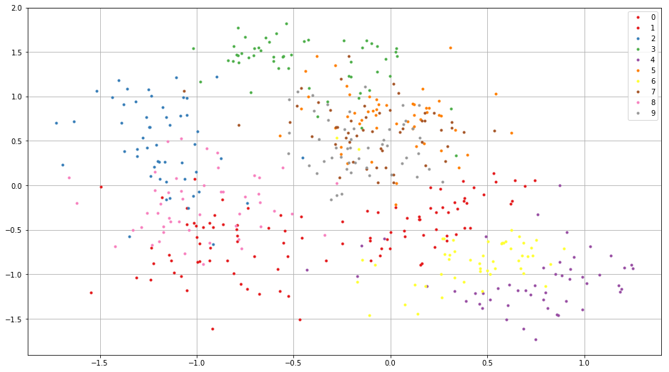
We visualize embedded training images as following. You see the images from the same class embedded near each other.

all_image = digits.images[:512, None]
all_label = digits.target[:512]

x_all = nn.Variable(all_image.shape)
x_all.d = all_image

with nn.auto_forward():
    embed, _ = cnn_embed(x_all, test=True)

plt.figure(figsize=(16, 9))
for i in range(10):
    c = plt.cm.Set1(i / 10.)  # Maybe it doesn't work in an older version of Matplotlib where color map lies in [0, 256)
    plt.plot(embed.d[all_label == i, 0].flatten(), embed.d[
             all_label == i, 1].flatten(), '.', c=c)
plt.legend(map(str, range(10)))
plt.grid()

Appendix

A. Logistic Regression

Here we demonstrate how to train the simplest neural network, logistic regression (single layer perceptron). Logistic regression is a linear classifier \(f : {\cal R}^{D\times 1} \rightarrow {\cal R}^{K\times 1}\)

\[\mathbf f(\mathbf x, \mathbf \Theta) = \mathbf W \mathbf x + \mathbf b\]

where \(\mathbf x \in {\cal R}^{D \times 1}\) is an input image flattened to a vector, \(t \in \{0, 1, \cdots, K\}\) is a target label, \(\mathbf W \in {\cal R}^{K \times D}\) is a weight matrix, \(\mathbf b \in {\cal R}^{K \times 1}\) is a bias vector and \(\mathbf \Theta \equiv \left\{\mathbf W, \mathbf b\right\}\). Loss function is defined as

\[\mathbf L(\mathbf \Theta, \mathbf X) = \frac{1}{N} \sum_{\mathbf x, t \subset \mathbf X} -log \left(\left[\sigma\left(f(\mathbf x, \mathbf \Theta)\right)\right]_{t}\right)\]

where \(\mathbf X \equiv \left\{\mathbf x_1, t_1, \cdots, \mathbf x_N, t_N\right\}\) denotes a dataset the network trained on, \(\sigma(\mathbf z)\) is softmax operation defined as \(\frac{\exp(-\mathbf z)}{\sum_{z \subset \mathbf z} \exp(-z)}\), and \(\left[\mathbf z\right]_i\) denotes i-th element of \(\mathbf z\).