Compress network by fixed point quantization

This tutorial introduces how to compress your network by fixed point quantization.

Introduction

Neural networks show reliable results on AI fields, such as object recognition and detection are useful in real applications. Concurrent to the the progress in recognition, the increase of IoT devices at the edge of the network is producing a massive amount of data to be computed to data centers, pushing network bandwidth requirements to the limit. Despite the improvements of network technology, data centers cannot guarantee acceptable transfer rates and response times, which could be a critical requirement for many applications. But CNN-based recognition systems need large amounts of memory and computational power, which perform well on expensive GPU-based machines, for example, AlexNet has 61M parameters (249MB of memory) and performs 1.5B high precision operations to classify one image. These numbers are even higher for deeper CNNs e.g.,VGG. They are often unsuitable for such edge devices, like cell phones, small devices and embedded electronics. Hence, reducing the storage of network and computation complexity is the task of optimization.

Currently, quantizing the weights and (or) input is the way which can dramatically reduce the memory and computation time and even keep original accuracy [1] (*).

This tutorial tends to share a few of experiments using nnabla for such optimitions.

Two approaches

There are mainly 2 approaches to design a fixed-point deep convolution network.

• Train a network with fix-point constraint

• Convert a pretrain float-point network to its fixed-point version

Binary Connect series functions, such as BinaryConnectAffine, BinaryConnectConvolution and Binary Weight series functions, such BinaryWeightAffine and BinaryWeightConvolution, fixed-point quantized series, such as FixedPointQuantizedAffine, FixedPointQuantizedConvolution acts as an important role for the first approach. These functions have different data paths for forward and backward. When forward, the float-point weights are converted to fixed-point weights or even binary weights, and the output is calculated by multiple such binary(quantized) weights with input. When backward, only float-point(or learnable) weights participate in the calculation of updating weights. In fact, binarizing weight is too extreme, fixed point quantization seems to be more commonly used.

Due to the second approach, a few steps need to be performed to keep minimal loss of accuracy. [2] provides a comprehensive analysis of such quantization for the relationship between quantization size and performance. Here, we shall do some experiments to illustrate the trade-off between accuracy and storage size.

We compared the ResNet23’s original version and the version using binary_weight_convolution(), we can observe the accuracy loss after using binary_weight_convolution(), which is worse than [3] mentioned. It should be possible to improve after more careful fine-tuning.

This tutorial only shows a basic way to compress network. There are still a lot of new approach not presented in this tutorial. For example, a new way is proposed as in [4], a quantization network is designed as a student network, a float-point high precision network is designed as a teacher network, the distillation technique is used to train to obtain the-state-of-art performance and accuracy.

The benchmark

We chose a simple network ResNet23 and CIFAR-10 dataset as the benchmark. First, let us obtain base metrics of this benchmark, such as accuracy, model size, and so on. The following shows the network structure:

Layer name	Shape	Required buffer size
conv1	(1, 3, 32, 32) -> (1, 64, 32, 32)	281344
conv2	(1, 64, 32, 32)->(1, 32, 32, 32)->(1, 32, 32, 32) -> (1, 64, 32, 32)	786432
conv3	(1, 64, 16, 16)->(1, 32, 16, 16)->(1, 32, 16, 16) -> (1, 64, 16, 16)	196608
conv4	(1, 64, 16, 16)->(1, 32, 16, 16)->(1, 32, 16, 16) -> (1, 64, 16, 16)	196608
conv5	(1, 64, 8, 8)->(1, 32, 8, 8)->(1, 32, 8, 8) -> (1, 64, 8, 8)	49152
conv6	(1, 64, 8, 8)->(1, 32, 8, 8)->(1, 32, 8, 8) -> (1, 64, 8, 8)	49152
conv7	(1, 64, 4, 4)->(1, 32, 4, 4)->(1, 32, 4, 4) -> (1, 64, 4, 4)	12288
conv8	(1, 64, 4, 4)->(1, 32, 4, 4)->(1, 32, 4, 4) -> (1, 64, 4, 4)	12288

To downsize the footprint, we should consider to downsize both the parameter size and variable buffer size, and especially prior for the maximal buffer size.

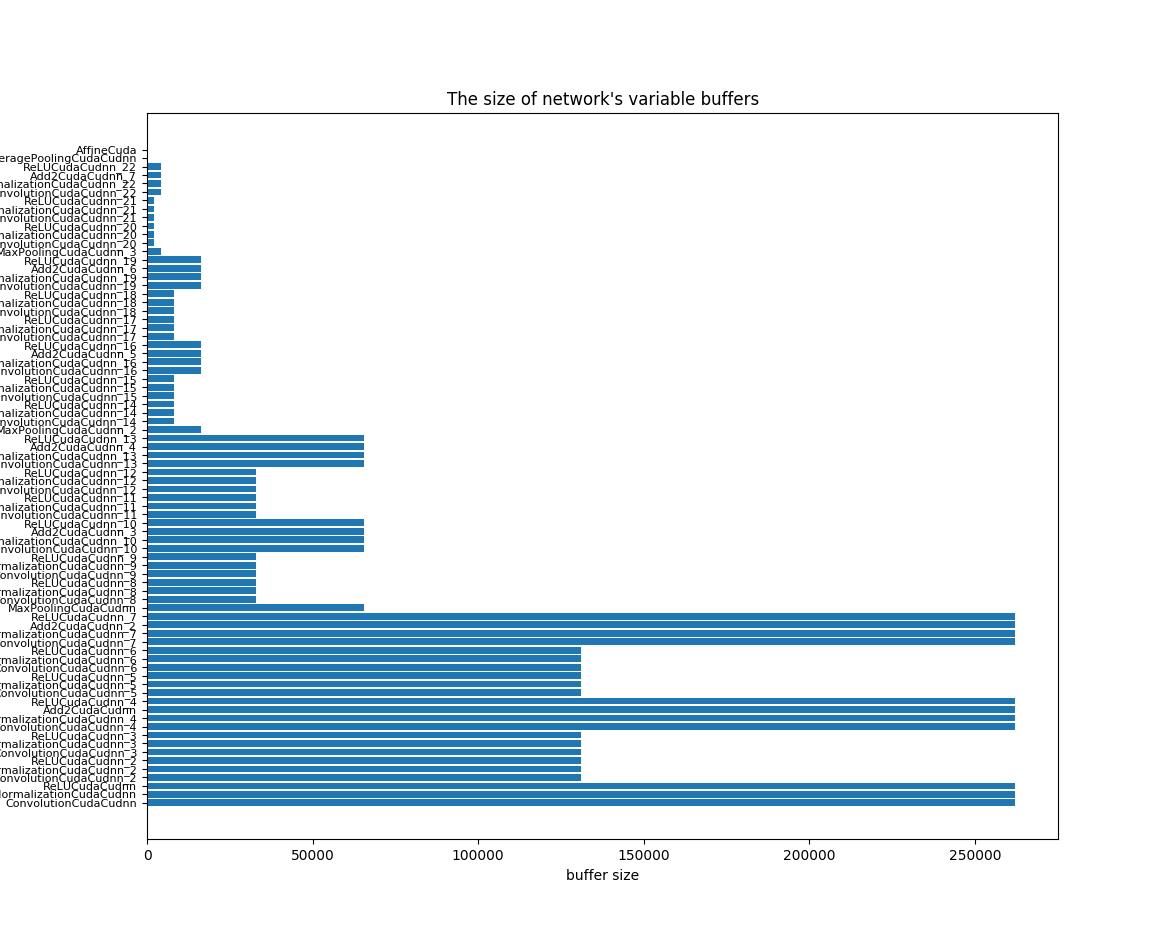
The network is created by the following code:

import nnabla as nn
import nnabla.functions as F
import nnabla.parametric_functions as PF

def resnet23_prediction(image, test=False, ncls=10, nmaps=64, act=F.relu):
    """
    Construct ResNet 23
    """
    # Residual Unit
    def res_unit(x, scope_name, dn=False):
        C = x.shape[1]
        with nn.parameter_scope(scope_name):
            # Conv -> BN -> Nonlinear
            with nn.parameter_scope("conv1"):
                h = PF.convolution(x, C // 2, kernel=(1, 1), pad=(0, 0),
                                   with_bias=False)
                h = PF.batch_normalization(h, batch_stat=not test)
                h = act(h)
            # Conv -> BN -> Nonlinear
            with nn.parameter_scope("conv2"):
                h = PF.convolution(h, C // 2, kernel=(3, 3), pad=(1, 1),
                                   with_bias=False)
                h = PF.batch_normalization(h, batch_stat=not test)
                h = act(h)
            # Conv -> BN
            with nn.parameter_scope("conv3"):
                h = PF.convolution(h, C, kernel=(1, 1), pad=(0, 0),
                                   with_bias=False)
                h = PF.batch_normalization(h, batch_stat=not test)
            # Residual -> Nonlinear
            h = act(F.add2(h, x, inplace=True))
            # Maxpooling
            if dn:
                h = F.max_pooling(h, kernel=(2, 2), stride=(2, 2))
            return h
    # Conv -> BN -> Nonlinear
    with nn.parameter_scope("conv1"):
        # Preprocess
        if not test:
            image = F.image_augmentation(image, contrast=1.0,
                                         angle=0.25,
                                         flip_lr=True)
            image.need_grad = False
        h = PF.convolution(image, nmaps, kernel=(3, 3),
                           pad=(1, 1), with_bias=False)
        h = PF.batch_normalization(h, batch_stat=not test)
        h = act(h)

    h = res_unit(h, "conv2", False)    # -> 32x32
    h = res_unit(h, "conv3", True)     # -> 16x16
    h = res_unit(h, "conv4", False)    # -> 16x16
    h = res_unit(h, "conv5", True)     # -> 8x8
    h = res_unit(h, "conv6", False)    # -> 8x8
    h = res_unit(h, "conv7", True)     # -> 4x4
    h = res_unit(h, "conv8", False)    # -> 4x4
    h = F.average_pooling(h, kernel=(4, 4))  # -> 1x1
    pred = PF.affine(h, ncls)

    return pred

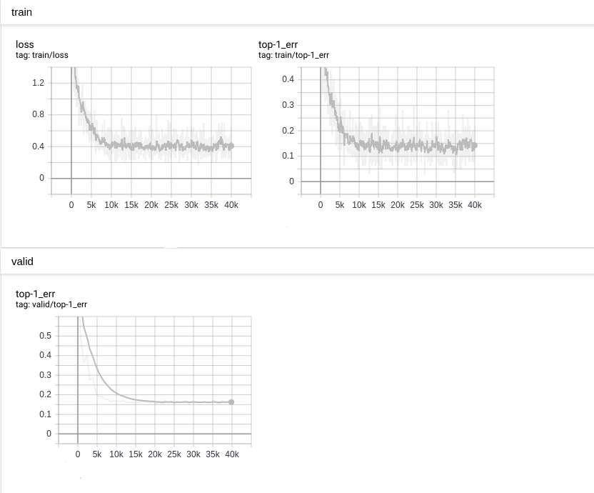
The top-1 error reaches to 0.16 as the following diagram:

We compared the accuracy between nnabla_cli infer and nnablart infer in CIFAR10 test dataset. The comparison code is as the following:

import numpy as np
import os
from cifar10_data import data_iterator_cifar10

data_iterator = data_iterator_cifar10
vdata = data_iterator(1, False)
iter_num = 100


def get_infer_result(result_file):
    d0 = np.fromfile(result_file, np.float32)
    d0 = d0.reshape((10, ))
    return np.argmax(d0)

def normalize_image(image):
    image = image.astype(np.float32)
    image -= np.mean(image)
    image_std = np.std(image)
    return image / max(image_std, 1e-5)


nnp_correct = 0
nnb_correct = 0
for i in range(iter_num):
    img, gt = vdata.next()
    img = normalize_image(img)
    img.tofile('input.bin')
    os.system('nnabla_cli infer -b 1 -c bin_class.nnp -o output_0 input.bin')
    os.system('./nnablart infer bin_class.nnb input.bin output_1')

    r1 = get_infer_result('output_0_0.bin')
    r2 = get_infer_result('output_1_0.bin')

    if r1 == gt:
        nnp_correct += 1
    if r2 == gt:
        nnb_correct += 1

    if r1 == r2 == gt:
        print("{}:  all same!".format(i))
    else:
        print("{}:  not all same".format(i))
print("nnp accuracy: {}, nnb accuracy: {}".format(
    float(nnp_correct) / iter_num, float(nnb_correct) / iter_num))

In this code, nnablart is an executable implemented based on nnabla-c-runtime. nnablart is a simple command-line interface, which can infer the network defined by *.nnb file. As we known, nnabla-c-runtime is a c implementation aims to small device with constraint memory, it contains carefully designed memory policy, and the code for training purpose is removed for saving memory. This test program iterates 100 samples, comparing with ground truth, figure out the accuracy.

...
NNabla command line interface (Version:1.0.18, Build:190619071959)
     0: input.bin
     1: output_1
Input[0] size:3072
Input[0] data type:NN_DATA_TYPE_FLOAT, fp:0
Input[0] Shape ( 1 3 32 32 )
Output[0] size:10
Output[0] filename output_1_0.bin
Output[0] Shape ( 1 10 )
Output[0] data type:NN_DATA_TYPE_FLOAT, fp:0
99:  all same!
nnp accuracy: 0.81, nnb accuracy: 0.81

binary_weight_convolution

We replaced PF.convolution() with PF.binary_weight_convolution() as the following:

import nnabla as nn
import nnabla.functions as F
import nnabla.parametric_functions as PF


def resnet23_bin_w(image, test=False, ncls=10, nmaps=64, act=F.relu):
    """
    Construct ResNet 23
    """
    # Residual Unit
    def res_unit(x, scope_name, dn=False):
        C = x.shape[1]
        with nn.parameter_scope(scope_name):
            # Conv -> BN -> Nonlinear
            with nn.parameter_scope("conv1"):
                h = PF.binary_weight_convolution(x, C // 2, kernel=(1, 1), pad=(0, 0),
                                   with_bias=False)
                h = PF.batch_normalization(h, batch_stat=not test)
                h = act(h)
            # Conv -> BN -> Nonlinear
            with nn.parameter_scope("conv2"):
                h = PF.binary_weight_convolution(h, C // 2, kernel=(3, 3), pad=(1, 1),
                                   with_bias=False)
                h = PF.batch_normalization(h, batch_stat=not test)
                h = act(h)
            # Conv -> BN
            with nn.parameter_scope("conv3"):
                h = PF.binary_weight_convolution(h, C, kernel=(1, 1), pad=(0, 0),
                                   with_bias=False)
                h = PF.batch_normalization(h, batch_stat=not test)
            # Residual -> Nonlinear
            h = act(F.add2(h, x, inplace=True))
            # Maxpooling
            if dn:
                h = F.max_pooling(h, kernel=(2, 2), stride=(2, 2))
            return h
    # Conv -> BN -> Nonlinear
    with nn.parameter_scope("conv1"):
        # Preprocess
        if not test:
            image = F.image_augmentation(image, contrast=1.0,
                                         angle=0.25,
                                         flip_lr=True)
            image.need_grad = False
        h = PF.binary_weight_convolution(image, nmaps, kernel=(3, 3),
                           pad=(1, 1), with_bias=False)
        h = PF.batch_normalization(h, batch_stat=not test)
        h = act(h)

    h = res_unit(h, "conv2", False)    # -> 32x32
    h = res_unit(h, "conv3", True)     # -> 16x16
    h = res_unit(h, "conv4", False)    # -> 16x16
    h = res_unit(h, "conv5", True)     # -> 8x8
    h = res_unit(h, "conv6", False)    # -> 8x8
    h = res_unit(h, "conv7", True)     # -> 4x4
    h = res_unit(h, "conv8", False)    # -> 4x4
    h = F.average_pooling(h, kernel=(4, 4))  # -> 1x1
    pred = PF.affine(h, ncls)

    return pred

The training become a bit slower and the accuracy loss can be detected. As the following:

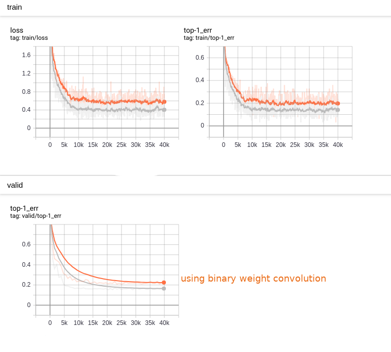
We saved the model and parameters as *.nnp file. Then, we shall convert it to *.nnb so that it can fit the memory-constraint device.

Reduce parameter size of *.nnb model

We need to set the data type of corresponding parameters, so that the binarized weights can be represented by SIGN data type.

Export a buffer setting file from our trained model

$/> nnabla_cli nnb_template bin_class.nnp setting.yaml

The output setting.yaml looks like:

functions:
  ...
variables:
  ...
  input: FLOAT32                          <-- buffer
  conv1/bwn_conv/W: FLOAT32               <-- parameter
  conv1/bwn_conv/Wb: FLOAT32              <-- parameter
  conv1/bwn_conv/alpha: FLOAT32           <-- parameter
  BinaryWeightConvolution_Output: FLOAT32
  conv1/bn/beta: FLOAT32
  conv1/bn/gamma: FLOAT32
  conv1/bn/mean: FLOAT32
  conv1/bn/var: FLOAT32
  BatchNormalization_Output: FLOAT32
  ReLU_Output: FLOAT32
  affine/W: FLOAT32
  affine/b: FLOAT32
  output: FLOAT32
  ...

We annotated buffer and parameter type based on its name character. The different between buffer and parameter is that: buffer value is undetermined at this time, while parameter values is determined. The quantization policy is different. As we known, conv1/bwn_conv/W is the float version, will not be used, just omit this. We need identify conv1/bwn_conv/Wb to be “SIGN” type, it looks like:

functions:
  ...
variables:
  ...
  input: FLOAT32
  conv1/bwn_conv/W: FLOAT32               <-- omit
  conv1/bwn_conv/Wb: SIGN                 <-- identified as SIGN
  ...
  output: FLOAT32
  ...

We tested the top-1 error in test dataset as the following:

nnp accuracy: 0.76, nnb accuracy: 0.73

As we can see, accuracy loss is trivial compared with its float version.

And the *.nnb size is reduced from 830KB to 219KB.

binary_connect_convolution

We replaced PF.convolution() with PF.binary_connect_convolution() and do same training as above.

The training become a bit slower and the accuracy loss can be detected. As the following:

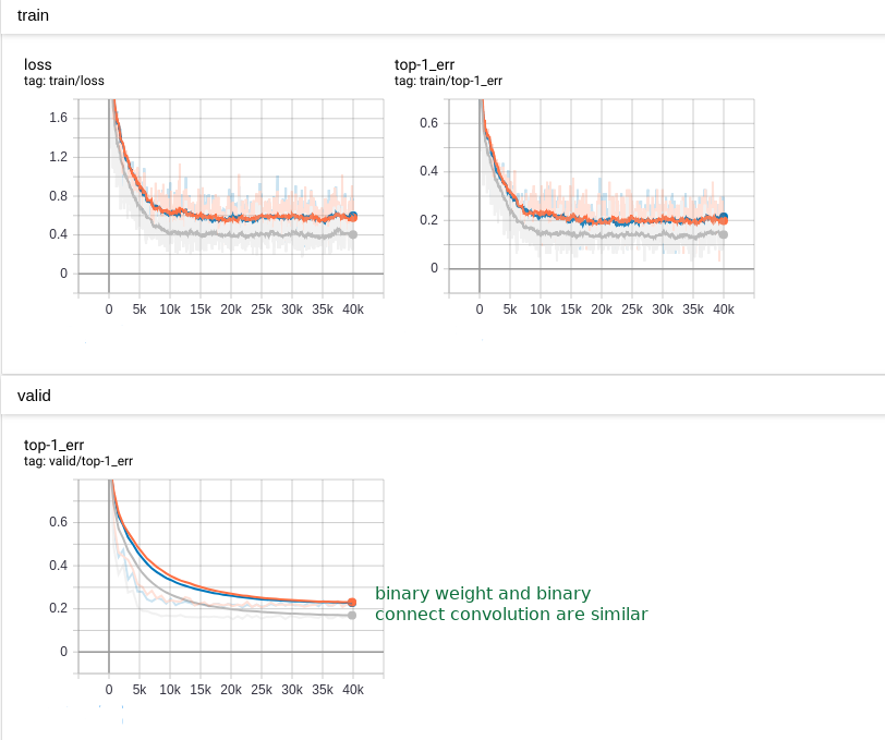
We tested the top-1 error in test dataset as the following:

nnp accuracy: 0.68, nnb accuracy: 0.71

As we can see, accuracy loss can be observed, but nnabla_cli got worse result than nnablart. From this test result, we found float32 version worse than binary quantized version. That seems a problem. The reason might be since the training process passes the data through 2 data paths, the binary weight data path has lower loss that the float32 data path at the same time.

Quantization functions

The mainly difference between binary_weight series functions and binary_connect series functions is the quantizing formula:

For binary_weight_convolution or binary_weight_affine:

\[\alpha^*=\frac{\sum{|W_i|}}{n}=\frac{1}{n}\|\mathbf{W}\|_{\ell_1}\]

\[\begin{split}B=\left\{ \begin{array}{ll} +1 & if \ \ W \ge 0 \\ -1 & if \ \ W < 0 \end{array} \right.\end{split}\]

\[W \approx \alpha B\]

For binary_connect_convolution or binary_connect_affine, there are 2 alternative binarization operations, one is:

\[\begin{split}W_b= \left\{ \begin{array}{ll} +1 & if\ w \ge 0 \\ -1 & otherwise \end{array} \right.\end{split}\]

Another way is:

\[\begin{split}W_b= \left\{ \begin{array}{ll} +1 & if\ with\ probability\ p=\sigma (\omega ) \\ -1 & if\ with\ probability\ 1 - p \end{array} \right. \\\end{split}\]

where sigma is the “hard sigmoid” function,

\[\sigma (x) = clip(\frac{x + 1}{2}, 0, 1) = max (0, min(1, \frac{x+1}{2}))\]

In nnabla implementation, binary_connect_xxxx() implements the following formula:

\[\begin{split}W_b=sign(W) = \left\{ \begin{array}{ll} +1 & if \ \ W > 0 \\ 0 & if \ \ W = 0 \\ -1 & if \ \ W < 0 \end{array} \right.\end{split}\]

According to this experiment, the accuracy is a bit different:

	Accuracy inferred by nnabla	Accuracy inferred by nnablart	Model size
float point	0.81	0.81	449.5 KB
using binary weight convolution	0.76	0.75	52.1 KB
using binary connect convolution	0.68	0.71	47.3 KB

The model size has already been cut-down about 10x dramatically.

Further reduce footprint

In order to keep maximal accuracy and reduce footprint as much as possible, let us try the second method as mentioned before. This method tends to work based on a pretrained network. Quantization process is done after training. Here, we chose the float-point trained model and start our experiment.

As previous analysis, we knew that the big share of footprint in this benchmark network is buffer size. As the following diagram, a circle represents a variable buffer, a rectangle represents a function. When perform function 1, buffer 1, buffer 2 and buffer 3 are occupied. After performing function 1, when function2 is performed, buffer 1 and buffer 2 are released, and this function’s output reuse buffer 1 if the size of buffer 1 can hold the data of function 2’s output.

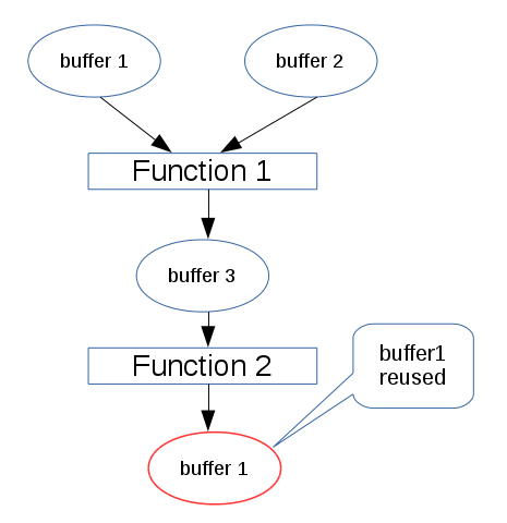
This buffer-reuse policy has been implemented during converting from *.nnp to *.nnb. The maximal of the occupying memory for each function represents the maximal footprint memory for inferring this network. In order to reduce this size, we may use quantization data type for variable buffer. As previous setting.yaml, if the following buffer type is changed, when converting from *.nnp to *.nnb, the buffer size will be calculated based on this new buffer type definition.

functions:
  ...
variables:
  ...
  input: FLOAT32             ==> input: FIXED8
  conv1/bwn_conv/W: FIXED8
  conv1/bwn_conv/Wb: FIXED8
  ...
  output: FLOAT32
...

As we known, this quantization process introduce quantization noise to the network, which sometimes cause obviously loss of the accuracy. How to choose best quantization step size, you may refer to [2].

Determine the fixed-point position

In converting from *.nnp to *.nnb, the fixed-point position can be determined automatically when quantizing parameter type, since the histogram(or distribution) is known at that time. Due to the fixed-point position of the variable’s buffer, in order to keep distortion as little as possible, we should determine its fixed-point according to its histogram (or distribution). But it is hard to know exactly the distribution of each of variable buffer, even though we statistics during training time. We supposed future test dataset has same distribution as current known dataset, make fixed-point decision based on the collection of current known dataset.

Manually tuning the fixed-point position is a work like an art. We shared some experience here. But an intelligent and automatic method seems be necessary.

As the following diagram, we collected the variable buffer’s distribution in a small known dataset. (Not all variable distribution are listed here.)

The distribution of buffer values

Of course, the simplest way to determine fixed-point position is only to dump the minimal and maximal value that occurs in variable buffer, but doing so might cause the value range is enlarged for values that some seldom occurs, then, cause precision loss of decimal part.

According to this distribution, we calculated the FP_POS as the following: (new_setting.yaml)

variables:
  ...
  Convolution_3_Output: FIXED16_12  <-- Change data type according to value distribution
  conv2/conv2/bn/beta: FLOAT32
  conv2/conv2/bn/gamma: FLOAT32
  conv2/conv2/bn/mean: FLOAT32
  conv2/conv2/bn/var: FLOAT32
  BatchNormalization_3_Output: FIXED16_12
  ReLU_3_Output: FIXED16_12
  conv2/conv3/conv/W: FIXED8
  Convolution_4_Output: FIXED16_12
  conv2/conv3/bn/beta: FLOAT32
  conv2/conv3/bn/gamma: FLOAT32
  conv2/conv3/bn/mean: FLOAT32
  conv2/conv3/bn/var: FLOAT32
  BatchNormalization_4_Output: FIXED8_4
  Add2_Output: FIXED8_4
  ReLU_4_Output: FIXED8_4
  ...

After modifying new_setting.yaml, the following command is used to convert from *.nnp to *.nnb:

$> nnabla_cli convert -b 1 -d nnb_3 models/bin_class_float.nnp models/bin_class_f_fq.nnb -s setting/setting_f_fq.yaml

-d nnb_3 is necessary to enable memory saving policy. By tuning, we got the the-state-of-art result:

nnp accuracy: 0.81, nnb accuracy: 0.79

Summary

After the quantization of variable buffer, the footprint is reduced noticeably from 1.2M to 495.2K, and accuracy is almost the same, as shown in the following table:

	model size	footprint	accuracy
float-point model	449.5 KB	1.2 M	0.81
parameter-quantized	126.0 KB	1.0 M	0.81
parameter-and-buffer-quantized	126.0 KB	495.2 KB	0.79

Comparing these two ways, the second way shows better result on current nnabla’s implementation. The reason is currently nnabla does not support SIGN parameter mode, so binarization weights lose accuracy without gaining the best benefit of saving memory. Future work is needed such that float-point weight parameters are removed from *.nnb for binary series functions.

• Notice: Currently, all experiments focus on classification problem, and softmax operation has higher tolerance to quantization error. The testing against regression problem has not yet been performed, so the accuracy loss is still unconfirmed.